What's New?
4712: Added TrES-3b 2014.07.11 LC by Carballo; revised P; no changes to depth, length or shape.
What's New? is a web page that records
changes to the various AXA web pages.
Note: ' symbol indicates AXA fit
value, not the "official" value
To see the light curve plots for an exoplanet, click on the
exoplanet's name (if it shows a link).
To download an ephemeris spreadsheet (Excel) that shows transit
times for all the BTEs for an observer's site coordinates, click
here: BTE Ephem.
Abstract for the AXA Web Pages - An Early
Version
This web page is a "public domain" archive for amateur
observations of known "bright transiting exoplanets" (BTE),
where "bright" means V-mag < 14. My intent is to "preserve"
amateur observations at one convenient location and to promote
sharing exoplanet observations by many observers to help in the
search for anomalies that might lead to a greater understanding
of exoplanet systems. Some light curves (LCs) are of transits
and others are out-of-transit (OOT). The archive manager will
enhance the LC by correcting for temporal trends and air mass
curvature using the non-transit portion of data. A line-segment
fit will be superimposed on the LC measurements. Each LC will be
accompanied by a listing of mid-transit time, transit length,
transit depth and an indication of whether the transit was early
or late. A web page is devoted to each exoplanet, with the most
recent LCs at the top. Observers of TransitSearch candidates are
welcome to submit observations. It's OK that most of them will
be featureless; this is useful information. A web page is
devoted to LCs for TransitSearch candidates. Most of the
data on the AXA will be transferred to the Caltech NStED archive
in January, 2009, where it will be available for download and
viewing a few months later. The fate of this web page will
depend on how many of the AXA features are present at the
NStED/AXA (I wrote that before learning about the Czech ETD).
Links Internal to this Web Page:
Original
Purpose for this Archive
Observation
Submission Format
Sampe
of Archive Processed Product
Explosive Growth
of Exoplanet Discoveries
Patterns to Look For
Observing
Philosophy
Aperture
vs. Technique
Filter Choice
Defocusing
Comment on
Correcting LCs for Slope and Curvature
Practice
Images
Ground Rules for
Professional Use of Data Files
Future of AXA
Contributors
AXA
Submission Statistics
Software
Used Statistics
Related Links
Original Purpose for this Archive
This archive was created in 2007 becasuse at that time amateurs
had no place to submit their observations of exoplanet transits
where they would be preserved for posterity. Since it is
scientifically important to preserve a historical record of
transit light curves (LCs), and since LCs that are only present at
an individual observer's web page are unlikely to be preserved for
later use, there was an unmet need for an archive of amateur LCs
that presented them in a uniform format. Such an archive would
grow in value and could become a useful resource many years in the
future. Only a handfull of amateurs are associated with a
professional group of astronomers, where archives are preserved,
and their LC archive s are not in the public domain. The AXA was
opened for anyone to submit observations that were likely to be
added to the AXA web pages and maintained as a historical archive.
In 2009 I discovered that the Czech Republic Astronomical Society
had been downloading data files from the AXA and fitting their own
LC models for display, and that they also were inviting amateurs
to submit raw data files to their web site. This web site was
called the Exoplanet Transit Database, and since it was maintained
by an institution instead of an individual it was a more suitable
place for safely archiving data. I therefore discontinued
accepting data files in December, 2009, and I encourage all
amateurs to submit their data to the ETD. Occasionally I will
accept data for special observing projects, so the remainder of
the material on this AXA home page will be preserved.
The structure of the present archive allows for easy browsing for the purpose of visually searching for patterns that would otherwise be difficult to detect. I anticipate that professional astronomers with their own archive (not in the public domain) will glean information from this one as they search for patterns that can only be done with large amounts of LC data. In this way amateurs with good observing skills can contribute to the professional astronomy community's growing understanding of exoplanet systems, and possibly produce interest in anomalies that could lead to the discovery of additional exoplanets in the same exo-planetary system.
This web page describes how anyone who has observed an exoplanet, and produced a light curve (LC), can submit their observations and have them added to the archive. As the archive manager I will assess the quality of the data and if it looks acceptable (99% of submissions are acceptable) I will proceed to process it. Baseline systematics will be assessed and a fit to the data using a line-segment transit model will be over-plotted on the measured data points. The resulting LC plot will list mid-transit time, transit depth and transit length. Measured mid-transit time will be compared with an ephemeris predicted time. A notation may be made on the LC plot showing 2-minute RMS of the individual measurements.
When many transits are present on a web page devoted to an exoplanet, and ordered with the most recent LC at the top, it is easy to notice the following patterns: transists occuring early or late (implying a need for refining the orbital period), depths varying in a systematic way with filter (related to star spectral type and center miss distance) and transit length varying over time. Some of these patterns can be used by anyone to search for other exoplanets using mid-transit timing anomalies, called "transit timing variations" (TTV). Other patterns may justify a reconsideration of stellar limb darkening and center miss distance. A search for another exoplanet in the same system can also be performed using the OOT data that might contain small depth features that repeat with a different period than the main transits. Many archives exist with exoplanet transit information, but none are in the public domain, and perhaps none are structured in a way that is convenient to use for the purposes just mentioned. This web page is meant for those who are not associated with professional teams that maintain a "secret" archive.
This section used to include instructions for preparing a data
file for submission to the AXA, but it has been moved to a
separate web page: DataFormat. I'll
simply show an example of a properly formatted data file and refer
you to the above link for explanations.
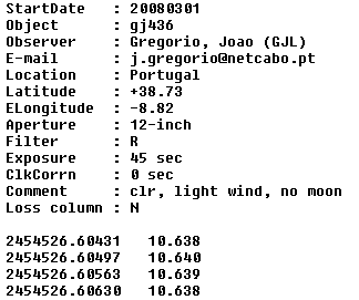
Sample data submission showing required format.
Here's an example of my preferred filename convention: 20080301-gj436-GJL.txt.
It conveys the information that the observations began on the date
2008 March 1 (UT), the object was GJ 436, and the observer's
3-letter "observer code" is GJL (details on the other web page).
Attach this file to an e-mail sent to:
a x a @ b r u c e g a r y . n e t
[remove spaces between characters]
Sample
of Archive Processed Product
Two light curve formats will be presented for each data
submission (starting May 1). There will be a top panel LC, a
bottom panel LC, and a 4-row information section between the
panels. In the following example the top panel is a version
of the data with the two principal systematic errors removed
(temporal trend and air mass curvature). This is the format used
by professional astronomers. Since amateurs have larger systematic
errors I have included the lower panel to show the same data
before removal of these systematic errors. The lower panel also
shows a air mass and "loss" plots (described below). For this
example we can readily see that the early data were made at very
high air mass, which explains the greater noisiness of the data
and extreme air mass curvature.
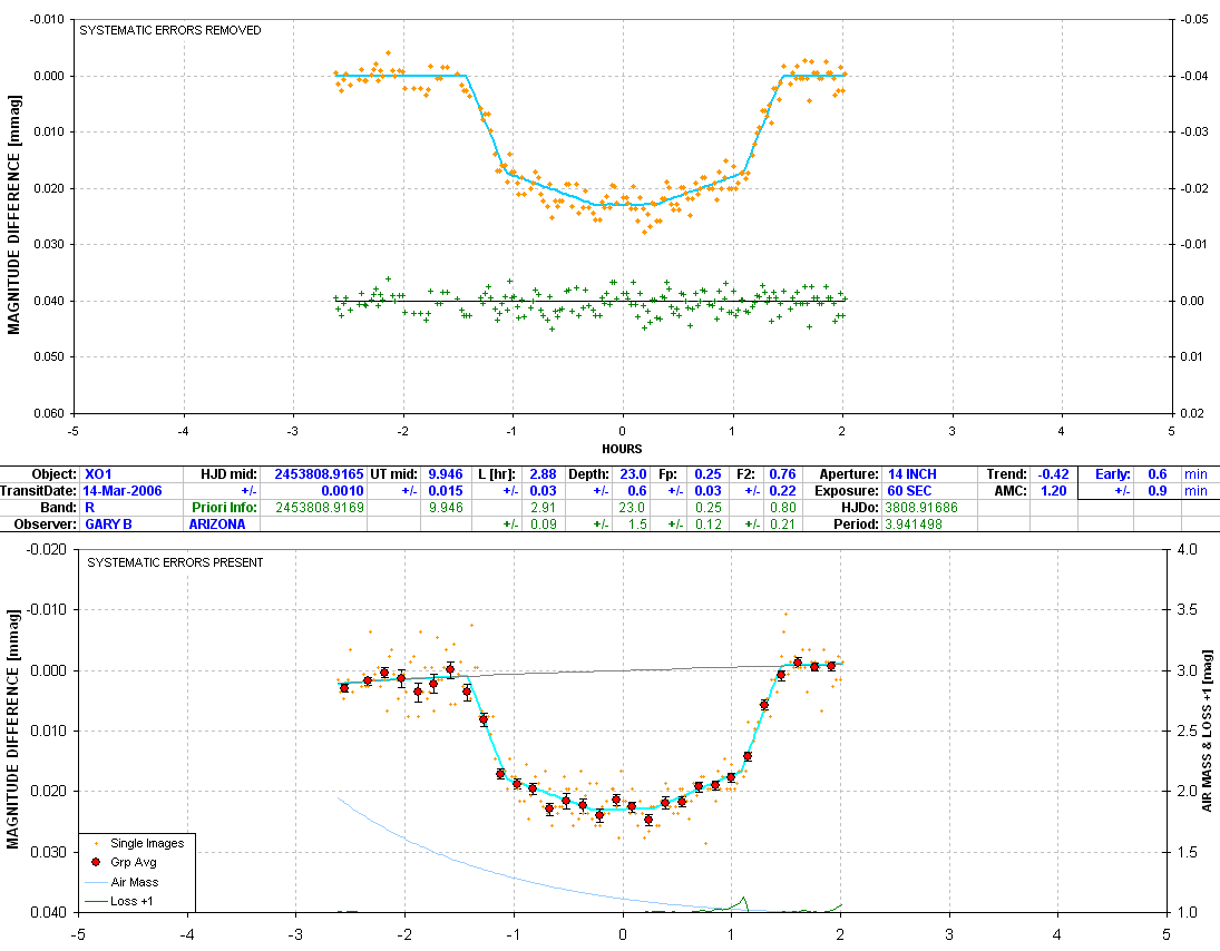
The middle section states that the transiting object is XO-1,
using a R-band filter, and mid-transit occurred on March 14, 2006
UT. The 7-segment model fit (explained in detail at model)
has a mid-transit HJD of 2453808.9165 ± 0.0010. This corresponds
to UT = 9.946 ± 0.015 (based on the date and source coordinates).
The ephemeris predicted HJD and UT are also shown in the 3rd row
(green). The transit length was measured to be L = 2.88 ± 0.03
hours, which is slightly longer than the consensus value of 2.91
hours. The transit depth is 23.0 ± 0.6 mmag, which is the same as
the consensus value. Fp is the fraction of time the transit is
"partial," defined using contact times as Fp = ((t2 - t1) + (t4 -
t3)) / (t4 - t1). The solution for Fp is 0.25 ± 0.03. F2 is the
ratio of depth at t2 and t3 divided by the depth at mid-transit,
and for this solution F2 = 0.76 ± 0.22. The ephemeris HJDo and
Period (used to calculate expected mid-transit time) are shown.
The fitted temporal trend (-0.42 mmag/hour) and air mass curvature
coefficient (+1.20 mmag / airmass) are given. The entry "Early: 0.6 ± 0.9 min" states that
mid-transit was earlier than the ephemeris time by 0.6 minutes.
You'll note that blue entries
are specific to the submitted observations and green entries are from an ephemeris
or a consensus of previous observations. The upper panel includes
a plot of departures of the measured magnitudes from the model
fit, or "O-C" (observed minus computed). The lower panel's large
red circle data, with SE bars, are averages of non-overlapping
groups of either 5, 7, 9, 11, 13 or 17 individual image values. At
the bottom of the lower panel is a green trace showing "losses"
offset so that their magnitude value is 1.0 when losses are zero
(as read on the right side). Losses refer to the effect of clouds,
dew on the corrector plate, wind shaking the telescope enough to
broaden the point-spread-functionof all stars so that some of the
photo electrons spill out of the aperture circle. For this example
there was dew formation on the corrector plate that was evaporated
with a hair dryer at 1.1 UT, and another dew formation just prior
to the end of observations (~0.1 magnitude loss in both cases).
I've adopted this presentation because it is quicker to produce
than previous versions. If Caltech really does assume
responsibility for the AXA it won't be open for public submissions
for at least 6 months, and during that time I want to minimize my
workload. A program is used to perform chi-square fitting of
submitted data and records a file that is easily imported to the
spreadsheet which is screen captured as an image file for import
to a web page. The entire process is much faster than the hand
solution searches I used to perform, and this will enable me to
accept more data submissions. If you preferred the other versions,
requiring hand-entered values for such things as mid-transit time,
length and depth, then I hereby apologize for abandoning them.
As stated above, a description is given of the very simple transit
"model" used for fitting the submitted measurements at model
fitting.
Explosive Growth of Exoplanet Discoveries
The number of bright transiting exoplanets has doubled in the past year (mid-2006 to mid-2007). There may be an equal number of undiscovered transiting exoplanets among the list of 246 exoplanets discovered spectroscopically (i.e., from radial velocity variations) found on the TransitSearch.org web site. There are plenty of observing opportunities for amateurs not associated with a wide field camera survey team, like the XO Project. Even an "arm chair" amateur astronomer can become engaged with a study of existing observations. There is merit in collecting all LC observations for each object and searching for patterns. One pattern would be transit timing variations (TTV) of mid-transit times; another would be a search for shallow transits during OOT times; and a search could even be made for LC structure within a transit or just outside transit by combining and averaging many LCs. For example, an exoplanet with rings may produce a brightening just before ingress and just after egress. Some day there may be a central archive where ALL exoplanet LC observations can be found. It is appropriate for either NASA or NSF to maintain such an archive. Caltech's IPAC archive would be an appropriate place for this addition. It would also be appropriate for a European institute to host the archive. Until this happens I would like to urge my fellow amateur astronomers to share their LCs on this public archive.
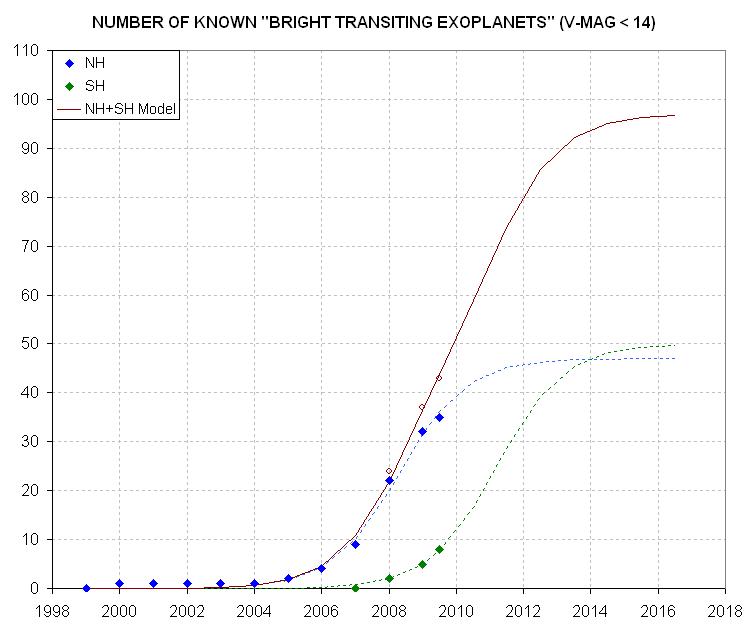
The cumulative number of "bright transiting exoplanets" in the northern celestial hemisphere (blue sybmols and model fit trace) grew exponentially with a doubling time of 1.1 years during the early years, and may be slowing, as this "sigmoid" fit suggests. Survey cameras in the summer hemisphere appear to be reproducing this curve with a 3 year lag (green symbols and model fit trace). The maximum number for each hemisphere can be different, as indicated. The total number (brown data and trace) could approach 100 in about 5 years.
The first 21 BTE discoveries were in the north celestial hemisphere because until recently the wide field search cameras were only in the Earth's northern hemisphere. Now that southern hemisphere cameras are in operation it won't be long before we'll know about as many BTEs in the southern skies. If we assume the discovery rate function for BTEs will be the same for each celestial hemisphere (cumulative number doubling time of 1.1 years before "saturation") then the cumulative number curve for the NH can be shifted ~ 2.9 years to show what can be expected for the SH . Before the list of northern sky BTEs is complete to 14th magnitude the discovery rate curve will flatten out to some unknown limit which will depend on how many long period exoplanets are there to be discovered. The "sigmoid" curve fitted to the NH BTEs suggests that this will happen in 2 or 3 years. But in the meantime, the SH discoveries will accumulate, causing the total number of known BTEs to reach asn asymtote of about 100 sometime in the next 5 to 10 years.
"Exomoons" is an exciting new thing to look for in amateur
transit observations, as pointed out by David Kipping (Sky
& Telescope, July 2009, pg 30-33; also described at the
author's web site: http://www.homepages.ucl.ac.uk/~ucapdki/exomoons.html).
The concept is simple: a moon of an exoplanet will cause it to
move around the parent star with a varying orbital velocity,
causing mid-transit timing variations (TTV) and also causing
transit length variations, TDV (Transit Duration Variations). TTV
effects for an Earth mass moon could be as large as 2 minutes, and
the TDV effect could be as large as 1 minute. These effects could
be measured by amateurs! Come on, AXA contributors, let's try to
find them!
If an exoplanet has a debris system in the same orbit (e.g.,
volcanic ejecta surrounding and perhaps following the "hot
Jupiter" planet) the debris particles will "forward scatter " and
produce brightness enhancements before ingress and after egress.
The pre-ingress and post-egress brightenings should have a
different brightening amount and shape. This effect is likely to
be too small for detection using amateur observations but
unusually large, transient ejection events should not be ruled
out.
If an exoplanet has a ring system the ring particles will also "forward scatter" and produce a brightening before ingress and after egress that can last several minutes. In 2004 Joe Garlitz and I independently noticed that amateur LC observations of TrES-1 showed a small brightening (~5 mmag) after egress, lasting ~10 minutes. Ron Bissinger did an exhaustive statistical analysis of many TrES-1 LCs and concluded that the feature was statistically significant. Subsequent HST observations failed to confrim the feature so we are left to assume that the apparent brightenings were a statistical fluke. All exoplanets should be inspected for such a feature even though the effect is probably going to be much smaller than amateur observations could detect (< 0.3 mmag according to Brown and Fortney, 2004 and Otha et al, 2008).
An exoplanet may have a moon of its own, and if its large enough it could produce a small fade either before ingress or after egress. This would probably be noticed as a change in mid-transit time since on any one transit the moon will affect only an ingress or only an egress for a given transit. Brown et al (2001) searched for this effect with HST observations of HD 209458 and found nothing. Again, amateur observations are likely to be insufficiently precise to observe such an effect unless the moon is comparble in size to the hot Jupiter.
Mid-transit time can vary if the exoplanet is accompanied by another exoplanet in an orbit with a period resonance, such as 2:1, 3:2, etc. For exoplanets with a long record of transit timing measurements these timing anomalies should be searched for.
Transit length and depth can vary if the transiting planet is close to "grazing" and another planet in a nearby orbit that inclined differently causes changes in the transiting planet's inclination. This was thought to be the situation for GJ 436 in January 2008 (Ribas et al, 2008a; Ribas has since withdrawn this suggestion in the light of later observations that offered a simpler interpretation). Still, any exoplanet with an "impact parameter" close to 1, such as GJ 436, TrES-2, TrES-3 and HD 17156, should be viewed as candidates for transit property changes due to inclination changes caused by another exoplanet in a resonant orbit.
If an exoplanet has Trojan planets (same orbital period but located at longitudes 60 ahead or behind) there may be a detectable fade at times that are offset 1/6 of a period before or after the main exoplanet transit event. For hot Jupiter periods of 3 days, for example, the Trojan features will occur ~12 hours before or after the ephemeris transit. This offset is longer than any single transit observing session, so only the OOT observations can be used for this purpose.
Sunspots will produce a small brightening during the interval Contact 2 to Contact 3 but they'd have to be large to be detected by amateur hardware. If a feature is seen on one LC it may not be seen on others unless the periods are the same (period of exoplanet orbit and period of rotation at the sunspot's latitude).
On a typical night at least one of the BTEs will undergo a transit. On those nights when none are observable check the TransitSearch candidate list. If no known BTE transits are on the schedule, and the TransitSearch candidate list is unappealing for the night, there is merit in conducting OOT observations of a BTE. Preference can be given to exoplanets that are ~1/6 of a period away from transit, since that's when Trojans would produce their transit signatures. Another consideration is "impact parameter" - the ratio of closest approach miss distance to star radius. Small impact parameters are good candidates for second exoplanet transits in outer orbits. Small impact parameter systems have flatter bottomed transit shapes (i.e., contact 1 to contact 2 is short compared with contact 2 to contact 3).
If your interest is in a search for LC transit shape anomalies, either brightenings or fadings before ingress and after egress, then give preference to observing a bright exoplanet. Although scintillation will be the same regardless of a star's brightness, the SNR (caused by Poisson noise) will be better for brighter stars.
May I suggest that you "adopt" an exoplanet that transists near
midnight and simply observe it every clear night. After inspecting
it for anomalies that you can hope are real and repeating with an
unknown period, the overall OOT shapes can at least be used to
learn about your observation's systematics. For example, an OOT
set of measurements would produce a LC that is "flat" and
"horizontal" if no systematics were present. However, if your
polar axis is slightly mis-aligned (>0.1 degree), and if your
master flat field is imperfect, the LC will have a sloping trend
of as much as several mmag per hour. If a small scale feature in
the master flat is imperfectly represented (such as a dust donut)
then features could be superimposed on the sloping trend line. A
hot or cold pixel (or imperfect master dark frame) could produce
the same features. Another systematic, that is quite common, is
for the OOT LC to be curved in a way that is related to air mass.
This arises when the exoplanet star is not the same color as the
reference star (or the average color of the reference stars, if
ensemble photometry is employed). If your OOT observations produce
an LC with a curvature that is correlated with air mass then you
may want to give attention to reference star color when choosing
reference stars.
I have slowly come to appreciate some fundamental differences
between the kind of variable star observing and image analysis
performed for the AAVSO versus that required for exoplanets.
Occasionally a new observer will be handicapped by adhering to
traditional variable star observing procedures. For these
observers I recommend reading a web page I created that describes
the observing task differences, and how observing strategy and
image analysis should be adjusted on behalf of the exoplanet task:
Exoplanet Stars Are Not Variable Stars.
Whenever someone asks "what hardware is needed for observing
exoplanet transits" I try to explain that a more relevant question
to ask is "how competent an observer must I be for observing
exoplanet transits?" This idea has been dramatically demonstrated
by an observation
that has recently come to my attention. Petr Svoboda (Czech
Republic) used a 1.33-inch aperture "telescope" (actually, a 34 mm
aperture camera lens) with a SBIG ST-7 CCD camera to obtain the
following light curve:
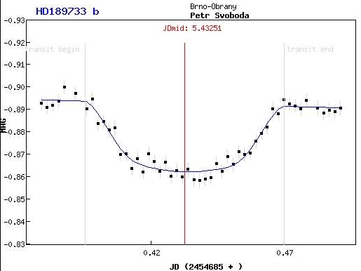
Small aperture light curve made with a 1.33-inch "telescope"
(34 mm camera lens).
Another impressive demonstration comes from Gregor Srdoc
(Croatia) who used a 2.5-inch camera lens attached to a regular
DSLR camera (12-bit) to measure a 9.5 mmag depth transit of XO-4.
The message from these two examples is that "aperture isn't
everything" because technique is important regardless of aperture.
Technique is based on an understanding of observing concepts,
image analysis and data analysis. I believe that it's difficult to
teach any of this because the best way to learn is to "flounder"
with whatever hardware is available! So my advice to anyone who
wonders what hardware is needed for exoplanet transit observing is
to change the question to "how willing am I to learn from
floundering with whatever hardware I have?" And remember, floundering
is fun!
An observing session that I designed specifically to identify the
best filter choice suggests that CBB-band (clear with
blue-blocking) is the best overall filter for exoplanet observing.
Details of this analysis are are given at FilterPlayoff.
I don't completely understand why defocusing can improve light
curve quality, but I have demonstrated to my satisfaction that for
the condition of a bright target star and a nearby interfering
star defocusing does indeed improve light curve quality. It will
be instructive for every serious observer to experiment with
defocusing. My demostration is at the following two web pages: DefocusingGeneralCase
& HD 80606
Defocused
Comment on Correcting LCs for Slope and Curvature
I disagree with the custom of professional astronomers who present transit light curve plots that have been "corrected" for a temporal trend and an air mass (extinction) correlation. The viewer has no clue about the magnitude of either correction when viewing a plot with those effects removed. As I show in my book Exoplanet Observing for Amateurs (Chapter 14, pg 82) the presence of these corrections influence such "transit parameters" as depth, shape, length and mid-transit time. There usually is a locus of points in slope/curvature parameter space (temporal slope and air mass coefficient) having equally good fits yet yielding varying results for transit parameters. Because of my experience with hand-fitting the LCs by experimenting with values for slope and curvature, and seeing the effect these choices have on transit parameters, I am reluctant to accept elaborate solutions for planet radius in a paper where there is no discussion of the slope/curvature fitting ambiguities. It's potentially misleading to simply experiment with the slope and curvature coefficients until the LC looks good, and then proceed with an elaborate chi-squared analysis seeking solutions for planet size, inclination, limb darkening, etc. without also including the slope and curvature coefficients as independent variables. Consider the following innocent-sounding description: "We then fit a linear function of time to the pre-ingress and post-egress data. A function of time proved to be a slightly better fit than the more traditional function of airmass." (reference available upon request).
I have adopted the practice of preserving the uncorrected photometry data points while applying the temporal trend and air mass correlated solutions to the "model fit" trace. These LCs may not look as pretty as the ones professionals publish, but they convey more information and are a more honest representation of the LC that was measured. Therefore, if you're used to seeing the pretty LCs with slope and curvature corrections removed, think twice before passing judgement on the sloped and curved LCs you see on the AXA web pages for each exoplanet.
I plan on adding a link to an illustration of quantitative
effects upon transit parameters when the slope and curvature
corrections are treated carelessly.
Several people have asked for a set of raw images of a real
exoplanet transit for the purpose of practicing with image
analysis and spreadsheet manipulation to achieve a useable transit
light curve. So, finally, I've created a web page where the images
can be downloaded. I've added some instructions (minimal) and a
sample LC to show what can be achieved from the images. The web
page is at PracticeImages.
Ground Rules for Professional
Use of Data Files
The description of various versions of these "ground rules" can be found at: GoundRules A short version that will be included in the header of those data files that are transferred to Caltech's IPAC computer (NStED archive), in late 2008, is presented here:
"Downloading of amateur data files is unrestricted. However,
since these data are unpublished it is recommended the observer
be contacted prior to use of data. The observer may be aware of
specific aspects of the data that should be taken into
consideration when interpreted, such as seeing, clouds, wind,
scintillation, clock-setting procedures, optimized photometry
apertures, etc. If these data are to be used in a publication,
it is requested that the observer be acknowledged by name along
with a brief description of the hardware used."
All good things come to an
end. I don't know how good the AXA has been, but I know that
it's coming to an end. Slowly. The ending is a good thing, for
it signifies the achievement of its original purpose. I created
the AXA 24 months ago to preserve amateur transit observations
in a convenient place where they could be used by professionals.
My intent has always been to persuade an institution to assume
these responsibilities. The AAVSO seemed like a natural place
for this but they couldn't afford it. I eventually persuaded
Caltech to become involved, but their role is limited to
archiving. The task of tabulating and analysing, yielding such
plots as TTV, depth and length for each transiting exoplanet,
remained to be addressed. This was labor-intensive and I sought
funding to automate it. NASA's Origins Program seemed
preoccupied with large, space-based projects, so I was facing
the prospect of toiling indefinitely with unpaid analyses and
plotting. I discovered by accident that the Czech Republic
Astronomy Society has been downloading AXA data files,
supplementing them with other data in the public domain, and
producing tables and plots that resemble those on the AXA (at a
web site called Exoplanet Transit Database, or ETD). The Czech
web site not only performs the analysis that AAVSO could not
afford, but they also accept data submissions and maintain an
archive. My goals of 18 months ago have been achieved and I can
begin to think about resuming that retirement that officially
began 10 years ago. It is a relief to know that institutions are
assuming the tasks that properly belong with them; it was risky
entrusting archiving of potentially valuable data with an
unfunded individual who is 10 years into retirement.
For the rest of this year,
2009, you may continue to submit data files to the AXA and I
will process them and post a light curve on the AXA. I will
convert these data files to the special format required by
Caltech's NStED archive, and transfer them to NStED for eventual
public domain access. By the end of 2009 the NStED will be able
to accept your data file submissions directly (using AXA
auto-fitting code translated to "C"), and at that time you will
switch from submitting to the AXA to submitting to the NStED. In
view of the fact that the Czech ETD is created mostly from
downloads of data that is originally submitted to the AXA (which
I convert to a standard format for downloading from AXA web
pages), when the NStED goes on-line (in mid-2009?) I assume that
the Czech ETD will obtain their data by downloads from the
NStED. Therefore, whenever you submit a data file to either the
AXA (or later to NStED) you can assume that it will also show up
at the Czech ETD, where it will be used to update tables of
observations and plots of TTV, depth and length. This is a good
arrangement because it relieves me from the tedious task of
manually updating tables and plots, and it solves the problem of
my inability to obtain funding to automate these tasks.
Incidentally, you have the option of submitting your data files
to only the Czech ETD, but then you wouldn't see my beautiful
plot with an auto-fit overlay, and your data would never appear
in the Caltech NStED. I therefore
suggest that you continue to submit data files to the AXA, as
before (even if you also submit to
the Czech ETD), and when the NStED
is ready to accept data files directly I will notify you about
this transition. If you want to see how your data compares with
other data, or if you want to see if your data is contributing
to an interesting TTV pattern, you may check the Czech ETD web
site. Here is a web address for the Czech ETD: Czech
Astronomical Society Exoplanet Transit Database
AXA
Submission Statistics - at Time of 500th Submission
(2009.05.19)
Two years ago this month I received an
e-mail from Joao Gregorio (Portugal) with a great-looking
transit light curve. Joao must have seen my name on the list of
amateurs who helped the XO Project discover XO-2 and XO-3, that
had been announced that month. I recognized observing talent,
more than comparable to that found among the dozen amateurs on
the amateur XO Extended Team. I had the following thought: "What
a shame if this LC, and the many others that were taken by
amateurs not on the XO extended team, were to fade from the
public domain and not be available for future generations of
professional astronomers wishing to study trends of transit
properties." This was the origin of my idea to start the AXA.
How fitting, therefore, that Joao Gregorio should be the one to
make the 500th submission of data to the AXA. Joao is now a
member of the XO Extended Team of amateurs, and he also
continues to contribute to the AXA. Congratulations, Joao!
During the 1.7 years that the AXA has
existed I have come to appreciate the strong interest in
exoplanet transit observing by amateurs in Europe. I would
occasionally ask at my favorite telescope store (Starizona, in
Tucson): "Your store is usually crowded with amateurs buying
things, yet as far as I can tell there are no amateurs in
Arizona observing exoplanets; so what are the amateurs doing
with the wealth of hardware that surely exists in the Tucson
area?" The answer was always something like "99.5% of amateurs
look through eyepieces, or use CCDs to take pretty pictures."
Suddenly, one day, this made sense. Americans are
"right-brained" and Europeans are "left-brained." Rather,
there's a slight preference of thinking styles in these two
directions, based on evidence that I won't bother you with here.
So, this prompted me to wonder about the statistics of
submissions to the AXA. Did some parts of Europe stand-out as
"hot beds" of exoplanet observing? And what about other regions
of the world?
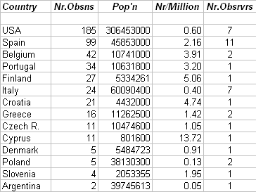
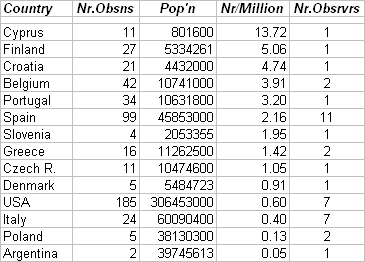
The first table, below, is a list of AXA
submissions by country, with the country populations and
calculated submission rates. The next table shows the same data
arranged by submission rate. Thanks to one observer in Cyprus
(Yenal Ogmen) this country has the highest per capita rate of
AXA submissions. The same explanation applies to Finland (Veli-Pekka Hentunen), Croatia (Gregor Srdoc), Portugal (Joao Gregorio) and
Slovenia (Matej Milelcic). Belgium has two active observers
(Tonny Vanmunster and Bart Staels). Keep in mind that in some
countries, such as Italy and the Czech Republic, amateurs have
other venues for posting their data, so my tables below will be
an under-count for them. Incidentally, most of the USA data are
from just two observers (removing them would lead to just 42 USA
observations, and a per capita submission rate of 0.14, the same
as Poland).
What about larger region statistics, such
as Europe and the USA? The table below summarizes world region
statistics.
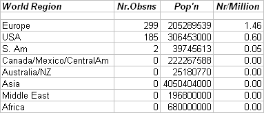
I'm surprised that no observations are
coming in from the most populous part of the world: China,
India, Russia and Southeast Asia (lumped together in the above
table as "Asia"). And what about Australia and New Zealand? Come
on, world, let's catch-up to Europe!
Finally, I just want to salute you
Europeans for your involvement with exoplanet observing and your
contributions to the AXA.
There are three main categories of software
used by exoplanet observers: hardware control, image analysis
and data analysis/display. The hardware will consist of the
telescope and CCD camera, and may also include a CFW, focuser,
autoguider, image stabilizer and dome (and maybe some exotics
others, such as cloud and rain sensors). Several observers used
different programs for control of the telescope and CCD. Image
analysis consists of calibrating (bias, dark and flat), star
field alignment, artificial star placement and photometry
readings of star flux (or magnitude). This last task may include
one or more stars for reference, or even an artificial star for
reference, and it may also include one or more check stars. The
third category is data analysis and display, which is almost
always performed in a spreadsheet, such as Excel.
Approximately 23 AXA contributors responded
to my inquiry about what software they used for the above tasks.
Here is my analysis of these responses.
Hardware Control: MaxIm DL (10),
TheSky (8), CCDSoft (5), AstroArt (4)
Image Analysis: MaxIm DL (8), FotoDif (5), Iris (5),
AIP4WIN (4)
Data Analysis/Display: Excel (15), GnuPlot (4)
I was surprised by the variety of programs
that are in use for the first two of these tasks. Some that were
mentioned only once aren't listed in the above summary.
The overall most-used software is MaxIm DL,
in spite of its high price. My
software usage is MaxIm DL, MaxIm DL and Excel. (I also use
TheSky/Six, but only offline, for monitoring target location
az/el and deciding where to position telescope for bright star
in autoguider FOV.)
AXA and TransitSearch contributors. TotNr is the total number of submissions since inception of the AXA (2 years ago). The Submissions (during past 12 months) is used to order the most active observers at the top of the list. For the group of observers with a total of more than 18 submissions during the past 12 months exceeds 18 the of listing within that group is determined by the date of earliest of these 18 submissions (right-most date), which is a way of showing who has been most active recently.
Total number of LC submissions...... 683
Active Observers & their Code Obs'g Site TotNr Submissions (during previous 12 months)*
Bruce
Gary
(GBL)
Arizona 104
1523,1309,0622,0622,0618,0507,0502,0429,0428,0426,0424,0421,0404,9927,9926,9924,9923,9917+
Gregor
Srdoc (SG2)
Croatia
81
0408,0415,0420,0426,0428,0429,9A03,9A03,9926,9926,9920,9910,9903,9903,9828,9830,9830,9828+
Joao
Gregorio (GJ2)
Portugal 51
1607,1401,1409,9B30,9A10,9A06,9A05,9A05,9720,9704,9626,9602,9601,9528,9528,9524,9524,9521+
Ramon
Naves
(NR2)
Spain
56
9908,9816,9815,9805,9729,9725,9720,9719,9718,9712,9612,9529,9527,9518,9406,9327,9324,9323+
Patrick Wiggins
(WPK) Utah
28
9B29,9B27,9B26,9B25,9B20,9B17,9B14,9930,9930,9922,9922,9821,9821,9818,9818,9818,9818,9810+
Colin
Littlefield (LCO)
Indiana, USA 18
9920,9920,9919,9913,9905,9811,9802,9727,9714,9708,9628,9626,9328,9302,9302,9227,9224,9215+
Veli-Pekka Hentunen (HVP)
Finland 30
0502,0419,9925,9327,9325,9308,9226,9105,9105,8a29,8b06,8b06,8b06,8b06,8b01,8b01,8b01,8a29+
Manuel
Mendez (MQZ)
Spain
37
9608,9518,9428,9414,9330,9316,9312,9119,9115,9114,8b25,8b16,8b14,8b11,8b06,8b01,8829,8825+
Bill Norby
(NWP)
Missouri 20
9825,9825,9817,9814,9807,9803,9801,9727,9723,9714,9630,9630,9626,9623,9619,9617,9605,9601+
Anthony
Ayiomamitis (AA2) Greece
23
0328,0328,9904,9828,9606,9514,8b26,8b22,8a08,8a05,8906,8903,8902
James
Roe
(ROE)
Missouri 28
9930,9930,8918,8918,8903,8819,8801,8808,8804,8729,8729,8729
Toni Scarmato
(SFI)
Italy 12
0502,0501,9626,9616,9426,9419,9328,9328,9326,8c06,8b20,8814
Johannes Ohlert
(OJ2)
Germany 9
9B05,9A09,9A09,9A09,9A09,9829,9829,9829,9808,9808,9705
Cindy
Foote
(FC2) Utah
59
9117,9117,9114,9109,8c11,8b18,8b17,8a29,8903,8903
Standa
Poddany (PS2) Czech
Republic 11
9B01,9426,9426,9408,9408,8a23,8905,8905,8827
Yenal
Ogmen
(OYE) Cyprus
11
9129,9129,9123,9121,8a11,8907,8922,8724
Fernando Tifner
(I32)
Argentina 7
9930,9930,9926,9922,9911,9328,8925
Joe Garlitz
(GJP)
Oregon 6
9828,9826,9728,9629,9624,9616
Paulo
Lobao (J15) Portugal
5
9713,9708,9703,9701,9630
Alessandro Marchini
(MXI)
Italy 5
9711,9415,9223,9202,9106
Fabio
Salvaggio+ (SFV)
Italy 8
9708,9703,9309,8901,8901
Enric Forne
(FE2) Spain
5
9731,8c16,8929,8929,8929
Ricard
Casas
(CRI) Spain
4 8929,8929,8929,8929
Brian
Tieman (TBJ)
Illinois 3
0415,0417,0418
Pere Salom
(B81)
Spain 3
9A30,9802,9726
Marcin
Wardak (WMK)
Poland 3
9429,9428,9425
Shawn Dvorak
(DKS)
Florida 3
9512,9512,9423
Bart Staels
(SBL)
Belgium 8
9215,9215,8c31
Peter
Kalajian (KP2) Maine
3
9711,8908,8911
Daniel Brown
(J06) United Kingdom 2
0503,0426
John Cordiale
(CQL) New York
2 9A21,9A02
Claudio Arena
(AC2) Italy
2
9713,9629
Xavier Puig
(PX2) Spain
2 9731,8929
Adam
Jesiokiewicz (JA2) Poland
2 9429,9428
Riccardo Papini
(PCC) Italy 2
9328,9206
Miguel
Rodriguez (RMU)
Spain 4
9322,880
Carlos
Gonzalez (B99) Spain
1 9711
Giuseppe Marino
(MG3) Italy
3 9525
Matej
Mihelcic (MHM)
Slovenia 2 9426
Giorgio
Corfini (CGI) Italy
1 9328
Claudio
Lopresti (LC3) Italy
1 9328
Javier
Salas (SJ2) Spain
1 9317
Enrique Garcia-Melendo (GM2) Spain
1 9314
Josep M
Coloma (CJI) Spain
1 8c16
Petr
Svoboda (SP2)
Czech Republic 1 8b03
Ramon
Costa (CR2) Spain
1 8929
Joal Bel
(BJ2) Spain
1 8929
Gustav
Muler
(MG2) Canary Islands 2 8914
Tonny Vanmunster (VMT)
Belgium
34
Darrel Moon
(MD2) Utah
3
Nicolaj Haarup
(HNI)
Denmark
5
Carballo, Juan-Luis
(GCJ)
Spain
1 4711
Stelios Kleidis
(KSM) Greece
1
* Date code is YMDD. Example #1: 20080317 = 8317; Example #2: 2007 December 31 = 7c31 (think HEX). Starting 2008 July 8 entries will be for date of submission, not observing date.
Some of the 3-letter observer codes for
the active observers have links to description of hardware
(and picture of hardware with observer).
RelatedLinks
Exoplanet
Observing for Amateurs (book, free PDF download)
Useful spreadsheets
(BTE_ephem.xls, etc)
Jean Schneider's Extrasolar Planet
Encyclopaedia
Greg Laughlin's TransitSearch
archive
Czech
Astronomical Society Exoplanet Transit Database (ETD)
NStED
(Caltech's NASA/IPAC/MSC Star and Exoplanet
Database)
Planetary
Society Catalog of Exoplanets
Bruce's
AstroPhotos
Resume
![]()
Artwork by Klaudia Einhorn
AXA
Logo Courtesy Matej Mihelèiè
(depicting transit of CoRoT-7)
WebMaster: B. Gary. This site opened: 2007 August 06, Last Update: 2016.03.26