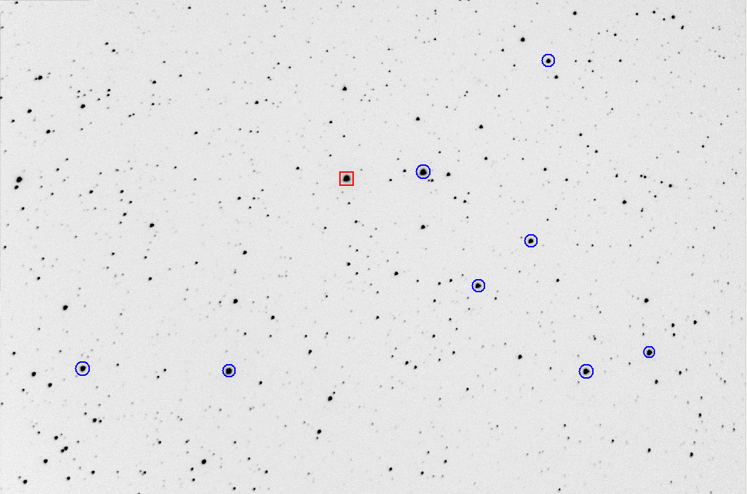
Figure 1. Star field surrounding target star (red square) and 8 reference stars. FOV = 31 x 21 'arc, north up, east left. FWHM ~ 3.0 "arc. (2009.01.31, median of seven 15-sec images)
This web page describes an evalutaion of the merits of defocusing to improve light curve precision.
Introduction
Bright stars require that either exposure time be reduced or defocusing
be employed. Otherwise the final light curve (LC) will suffer from low
duty cycle and therefore loss of precision per unit of pbserving time.
This web page describes an observing session of a 9th magnitude star that
employed various amounts of defocusing in an attempt to determine if there
was a best focus setting.
Glossary
dFOC = de-focus value; defined as the difference between
PAR75 for a defocused image and a sharply focused image
DutyCycle = fraction of observing time spent exposing
FWHM = full-width at half-maximum (applicable for
sharply-focused, unsaturated star image; expressed as either "arc or pixels)
IR1 = information rate, defined in a way that allows
for the easy calculation of precision [mmag] for a minute of observing
time.
LC = light curve
OOT = out-of-transit
PAR = photometry aperture radius (radius of inner
circle; usually expressed in units of pixels)
PAR50 = photometry aperture radius that encloses
50% of the star's total flux
PAR75 = photometry aperture radius that encloses
75% of the star's total flux
PAR98 = defined as radius of circle that contains
98% of defocused star's total flux
PSF = point-spread-function (regardless of focsus
setting)
px = pixel(s)
RMS1 = 1-minute equivalent RMS of individual LC
magnitudes (preferably, using the neighbor differences method)
The 1-min equivalence is calculated using RMS1 = RMSi * ( g [sec] / 1 minute)½)
where RMSi is RMS of individual images with exposure time g
Hardware
My telescope is a 11-inch aperture Celestron (CPC1100) mounted on an equatorial
wedge. I use a focal reducer and SBIG AO-7 image stabilizer in front
of a SBIG ST-8XE CCD camera. The AO-7 employs a tip/tilt mirror that
can be operated at several Hz, and when mirror motion exceeds a user-specified
limit a correcting nudge signal is sent to the telescope drive motors.
The polar axis has been aligned to the north celestial pole with an accuracy
of ~2 'arc. This assures that when the AO-7 keeps an autoguided star
fixed to a pixel location on the autoguider chip the star field does not
rotate about that star and simultaneously move the star field across
the main CCD chip. This arrangement assures that the star field is fixed
with respect to the CCD pixel field to within a few pixels during the
course of a many hour observing session. The image scale is 1.21 "arc/pixel,
and the FOV is 31 x 21 'arc. I use a wireless focuser (Craycroft type)
for adjusting the position of the optical back-end (the mirror is not moved).
MaxIm DL 5.03 is used to control the telescope, wireless focuser, AO-7
and CCD camera.
Each observer's hardware is different, and atmospheric seeing is different
each night, so the following is presented with the purpose of illustrating
concepts that can be used to guide observers in choosing optimum observing
and image analysis strategies.
Review of Usual Strategy for Sharply-Focused Exoplanet Transit
Light Curves
Normally, transiting exoplanet light curves are produced using sharply-focused
images and a photometry aperture radius (PAR) of about 3 x FWHM. Slightly
smaller and larger PAR values can sometimes produce small improvements
(e.g., PAR/FWHM within range 2 to 6). When a star is close to the target
star it may not be possbile to employ this standard PAR setting. Therefore
it is useful to know what penalties are incurred when very small values
for the PAR/FWHM ratio are employed.
Here's the star field used for this observating session (2009.01.31):
Figure 1. Star field surrounding target star (red
square) and 8 reference stars. FOV = 31 x 21 'arc, north up, east left.
FWHM ~ 3.0 "arc. (2009.01.31, median of seven 15-sec images)
Here's a sample light curve (LC):
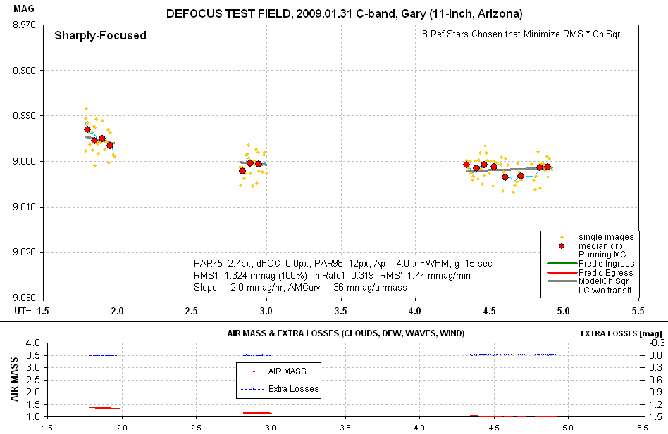
Figure 2. Light curve for sharply-focused images using
ApertureRadius/FWHM = 4.0. RMS1 = 1.324 mmag. Other parameters are described
in text.
The following figure is a plot of LC precision versus photometry ApertureRadius/FWHM
(i.e., PAR/FWHM):
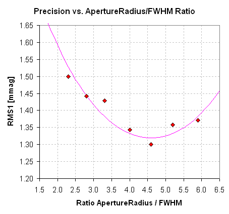
Figure 3. Precision versus ratio ApertureRadius/FWHM
for 2 hours of sharply focused observations (102 images).
Fig. 3 shows that for this set of sharply-focused images the "penalty"
for departing from the optimum PAR/FWHM = 4.5 is small. Using PAR/FWHM
= 2.3, for example, has a precision penalty of ~14%. This corresponds to
a 30% observng time penalty (since SNR is proportional to SQRT(ObservingTime)).
Defining Information Rate
Information rate should be defined such that doubling an observing session's
length doubles the information acquired (assuming no changes in seeing,
etc). When telescopes are compared using the information rate concept it
can be surprising to learn that doubling aperture will increase information
rate 16-fold. The way to understand this is to ask how much longer
the smaller telescope needs to observe to achieve the same SNR for a given
object. The telescope with half the aperture (diameter) has 1/4 the flux
of photons incident on the CCD compared to the larger telescope. The ratio
of SNRs is therefore 1/4 (assuming all other parameters are the same).
To overcome this SNR disadvantage the smaller telescope will have to observe
16 times longer. Hence, the ratio of information rates is a whopping 1:16!
This example illustrates the basic concept of information rate.
For a given telescope system it makes sense for the observer to exploit
all possible ways to maximize information rate. I want to define information
rate for use with exopanet LCs in a way that relates to the "gold standard"
of achieving a precision of 1 mmag per minute of observing time! Let's
call this version of information rate IR1, and when IR1 = 1 "minutes per
mmag" a precision of 1 mmag is achieved every minute of observing time.
Amateurs aspire to achieve IR1 = 1, and as far as I know never have, while
professionals aspire to never fall below IR1 = 1. An IR1 of 1.0 is what
separates amateurs from the professionals, due in large measure to differences
in hardware, observing site and software - but also due to differences in
knowledge about image processing and data processing. One of the purposes
for my tutorials is to "bridge this gap" and raise amateurs as much as possible
to the proficiency level of professionals.
Let's derive an equation for IR1 in small steps. First, consider that 4
images should contain 4 times as much information as one image, yet the RMS
of the average of 4 images is reduced to only 1/2 the RMS of one image. Thus,
information rate is proportional to 1 / RMS2. This is the first
term in a series of multiplicative terms.
Second, what's the effect of duty cycle on IR1? For reference consider
that duty cycle is ~ 1 (negligible download time, and no "settle time" for
autoguider reacquisition) and that 1-minute exposures occur every minute.
If individual 1-minute images exhibit a precision of 1 mmag, then IR1 =
1 [minutes per mmag]. This is how we're defining the scale for IR1. If, however,
duty cycle = 1/2, meaning that two minutes are required to get one image,
information rate is reduced to half the original value. Thus, IR1 is proportional
to duty cycle.
The product of the first two terms for information rate is then DutyCycle
/ RMS12, where RMS1 is the precision for 1-minute exposure
images.
Third, consider the case in which 2-minute exposures exhibit 1 mmag precision
per image. If the exposure time was reduced we know that RMS would increase.
If the exposure time was reduced from 2 minutes to 1 minute the simplest
calculation is that each image would exhibit an RMS precision that is root-2
higher, i.e., 2½ = 1.414 [mmag/min]. In other words, to
convert precision to 1-minute equivalent exposures we may use the equation
RMS1 = RMSi × g [minutes] ½, where RMSi is the RMS
for individual images with exposure time g. Note that the term in the previous
step is 1 / RMS12 , so this term can be written 1 / ( RMSi2
× g [minutes]).
Combining terms yields: IR1 = DutyCycle / ( RMSi2 × g [minutes])
Referring back to Fig. 2, a LC for sharp-focus images, RMS2 = 0.95 and
DutyCycle = 15 / (15 + 8 + 4) = 0.555. Therefore,
IR1 (sharp-focus) = 0.555 / ( 0.952
× 2 )
= 0.555 / 1.80
= 0.308
which means that each minute provides only 41% of the information needed
to achieve a precision of 1 mmag per minute. This is equivalent to stating
"To achieve 1 mmag precision requires 2.4 minutes (1 / 0.41) of telescope
time." Another equivalent statement is "Each minute produces a precision
of 1.56 mmag (1 / 0.41½ )."
The 15-second, sharp-focus images did not meet the desired goal of IR1
= 1.00, corresponding to 1 mmag precision each minute, but it does represent
a level for IR1 that must be improved upon by defocusing in order for
the defocusing strategy to have merit (for this target, hardware and observing
condition).
As an aside, it is often stated that a purpose for defocusing is to reduce
the effect of scintillation. Longer exposures reduce scintillation for individual
images, to be sure, but whereas this improves RMSi it has only a small
effect on RMS1, and hence information rate. The only benefit provided by
the longer exposures is from an improved duty cycle. The very same argument
applies to Poisson noise, which is also reduced for longer exposures, but
again, this only improves RMSi and has only a small effect on RMS1, and hence
information rate. The benefit is purely from a better duty cycle afforded
by longer exposures. The thing to optimize is not RMSi, but IR1!
Defocus Observations
Three questions have to be answered when considering employing a defocusing
strategy:
1) When should defocuing be employed?
2) How much should you defocus?
3) How large a photometry aperture is optimum
for processing the images?
Faint targets shouldn't be defocused. For example, asteroid observing requires
careful attention to focus in order to merely locate the asteroid for image
processing. Bright targets can "require" defocusing in order to avoid extremely
poor duty cycles. I'm going to address these questions in reverse order for
the simple reason that the rest of the analyses will go faster. So first
we'll determine a "rule" for setting the photometry aperture, then we'll
figure out how much to defocus for a given star and finally we'll decide
when to employ defocusing for "medium bright" stars.
Best Photometry Aperture Size
I'll use observations of another star field and another date to assess
optimum photometry aperture radius (PAR) for images that are defocused
enough to produce donut-shaped PSFs. One reeason for this is the desire
to use a long stretch of data for adequately assessing whether a given PAR
is better than ofther choices. On 2009.02.01 I observed HD 17156 continuously
for 3 hours with a highly defocused setting. Focus was offset "out" a fixed
amount and was updated using automatic temperature compensation in order
to maintain the same defocus amount throughout the observing session. For
these images the outer edge of the donut pattern had a radius of 12 pixels.
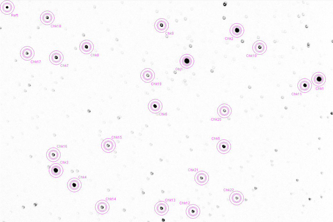
Figure 4. FOV of HD 17156 ("Obj") star field showing "donut"
shapes and a photometry aperture radius much larger than the donut. FOV
= 21 x 31 'arc, north up, east left. (2009.02.01)
There were 291 images, each exposed 30 seconds, which kept 8.17 V-magnitude
HD 17156, the brightest star, below saturation (peak ~30,000 counts).
Photometry measurements were made with PAR = 10, 12, 14, 16, 18 and 20
pixels. For each aperture radius an extensive procedure was used to select
the best reference stars from among the 22 candidates. Outlier data were
rejected in a way that maintained acceptance of 99% of the images. In effect,
the final reference star selection was based on which set yielded the lowest
noise and best fit to a simple model. Since this was an OOT observation
the model consisted of a slope and air mass curvature (and offset). Following
is the light curve for the 14-pixel radius fit.
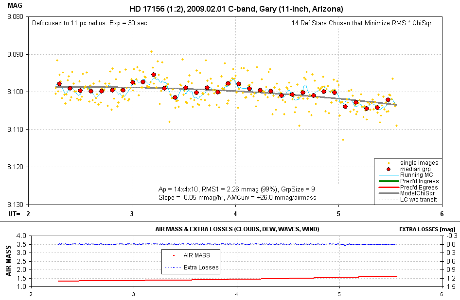
Figure 6. Light curve for the photometry aperture radius
choice of 15 pixels after solving for a best fit (i.e., best choice of
reference stars and model slope, air mass curvature and offset).
This LC has RMS1 = 2.26 mmag. Since DutyCycle = 0.71, IR1 = 0.14 (i.e.,
0.71 / 2.262). This is smaller than for the previous night, when
IR1 = 0.32, due perhaps to greater air mass (hence worse seeing) and possible
a greater level of scintillation.
The following plot shows "RMS with respect to the best fitting model"
versus photometry aperture radius.
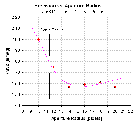
Figure 7. Dependence of RMS precision on photometry aperture
radius (PAR) for highly-defocused, donut-shaped PSF .
Based on this one case study the following "rule" suggests itself:
Optimum Photometry Aperture Radius
= 1.30 ×"PSF Donut-Shaped Outer Edge Radius"
But wait, we have more ground-work before adopting a rule for estimating
an optimum PAR. The above rule only applies to highly-defocused iamges;
we need to address the matter of slightly-defocused images. Hopefully we
can discover a universal principle that related optimum PAR to FFR for all
images, regardless of focus.
Estimating Optimum PAR
So far I've shown a way to estimate optimum PAR for sharply-focused images
and highly-defocused images, summarized here:
Optimum PAR = FWHM ×4 for sharply-focused images,
and
Optimum PAR = 1.3 × Radius to Outer Edge of
Donut-Shaped PSF for highly-defocused images.
What about slightly-defocused images? It sure would be handy to have a
"rule" that applies to all three focus regimes.
Consider a bright star in sharp focus, and let's ask the question "How
does flux vary with PAR?" Here's the answer for one of my sharply-focused
images:
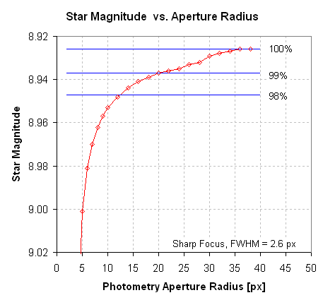
Figure 8. Star magnitude versus PAR. 98% of the star's flux
is contained within a radius of ~12 pixels.
It's surprising that flux within an aperture circle just keeps increasing
well beyond where visual inspection thinks star flux exists. The next image
has circles enclosing 98%, 99% and 100% of the star's total flux.
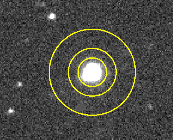
Figure 8. Bright star used to determine FFR. The inner circle
encloses 98% of the total star flux (PAR=12 px), the middle circle encloses
99% (PAR=20 px), and the outer circle includes ~100% (PAR=36 px). FWHM
= 2.6 pixels, or 3.2 "arc. (I pixel edited to remove an interfering
star below the target star.)
Referring back to Fig. 3, where it is shown that the optimum PAR ~ 4.5
× FWHM, we surmise that if a flux percentage is to be used to estimate
optimum PAR we might use the 98% criterion (referring to Fig. 7).
The suggestion, therefore, is that instead of estimating optimum PAR from
FWHM we instead determine what PAR produces 98% of the star's total flux.
I wonder if this criterion would also work for highly-defocused stars?
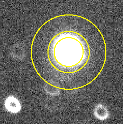
Figure 9. Highly-defocused image with circles placed to
correspond to 98%, 99% and ~100% of the star's flux. The PAR values are
14, 20 and 36 pixels.
Note that the 98% flux circle is achieved for PAR = 14 pixels. Referring
back to Fig. 7 this is the PAR we want for optimum precision! So,
"Optimum PAR can be established
by determining what PAR value encloses 98% of the star's flux for both
sharply-focused and highly-defocused images."
This is convenient! Note that optimum PAR for sharply-focused and highly-defocused
stars is about the same: 12 and 14 pixels. It is tempting to assume that
partially-defocused images will have an optimum PAR of ~13 pixels. This
is a reasonable speculation because the PSFs for the three focus regimes
will increase in size uniformly with increasing defocus. I hereby adopt the
above "rule" for determining optimum PAR.
Definition of Defocus Amount: Defocus75
Based on the success of the previous exercise for determining optimum PAR
from percentage flux measurements, I hereby propose to define a parameter
based on the 75% of total flux circle for use in quantifying how much defocus
is present in an image. Let's give this paramater a name, PAR75. Consider
the following three images:
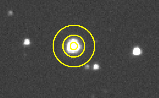
Figure 10. Sharply-focused image, with PAR75 = 2.7 px (inner
circle is PAR = 3 px). FWHM 2.4 pixels (2.9"arc). FOV =
2.5 x 1.6 'arc.
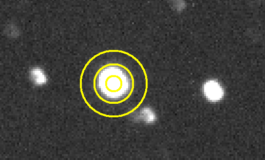
Figure 11. Slightly-defocused image, with PAR75 = 4.3 px
(inner circle is PAR = 4 px).
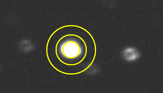
Figure 12. Highly-defocused image, with PAR75 = 6.5 px (inner
circle is PAR = 7 px).
For this observing session (2009.01.31), and for my hardware (image scale
1.21 "arc, etc), the sharpest possible image has PAR75 ~ 2.7 px. If we
subtract this value from any other image's PAR75 we will have a measure
of the defocus amount. For the above three images, we have:
dFOC = PAT75 - 2.7 px (for this observing session, 2009.01.31)
dFOC = 3.8 px for the highly-defocused image
dFOC = 1.6 px for the slightly-defocused image
dFOC = 0.0 px for the sharply-focused image
Light Curve Precision versus Defocus Value
We're now ready to analyze images with different amounts of defocusing and compare precision with the amount of defocus.
On 2009.01.31 I observed the 9th magnitude star described in the above
section, "Review of Usual Strategy for Sharply-Focused Exoplanet Light
Curves." For each of the 10 defocus settings I observed for 10 minutes,
using 15-second expsoure times. About 30 images are available for analysis
for each defocus setting. We have already seen the LC precision for sharply-focused
images (Fig. 2). The precision is ~0.95 mmag per 2-minute equivalent
exposure. Our goal is to determine how much better we can do by defocusing.
Let's begin with a highly-defocused set of images from the 2009.01.31 observing
session. In the following table "Focus Set'g" is listed in terms of whether
the focuser is in "i" or out "o" with respect to a sharp focus setting.
Focus dFOC RMS1
Set'g px mmag
i55 2.9
1.80
i45 2.4 1.86
i30 1.7 1.69
DF0 0.0 1.32
o20 1.2 0.96
o30 1.8 1.02
o45 2.6 1.26
o55
o65
o75
There's a smooth pattern of RMS1 versus focus setting that favors a slight defocus in the "out" direction. A slight defocus in the "in" direction has greater RMS1.
[more coming...]
Why?
I used to think that the only reason for defocusing was to improve duty
cycle. But compare the "sharply focused image set with large aperture" with
"defocused image set with large aperture" (same apertures), and the RMS
per 2-minute equivalent image, unadjusted for duty cycle, is better for
the defocused image than for the sharp image. The two precisions are 3.09
mmag per image and 2.02 mmag per image. Since duty cycle has nothing to
do with these two precision calculations there's something going on that
has to do with the spreading out of where photo-electrons are produced.
Could it be that when most of the star's photo-electrons originate from
only a few pixels that the readout noise per pixel, or the thermal noise
per pixel, has a greater percentage effect on the total flux than when many
pixels are involved? When most of the photo-electrons come from just a few
pixels could small errors in the flat field contribute a greater error in
the total flux than when these flat field errors are averaged-out over more
pixels? Could someone help me understnad this?
Conclusion
____________________________________________________________________
WebMaster: B.
Gary.
Nothing on this
web page is copyrighted. This site opened: 2009.01.31. Last Update: 2009.02.09