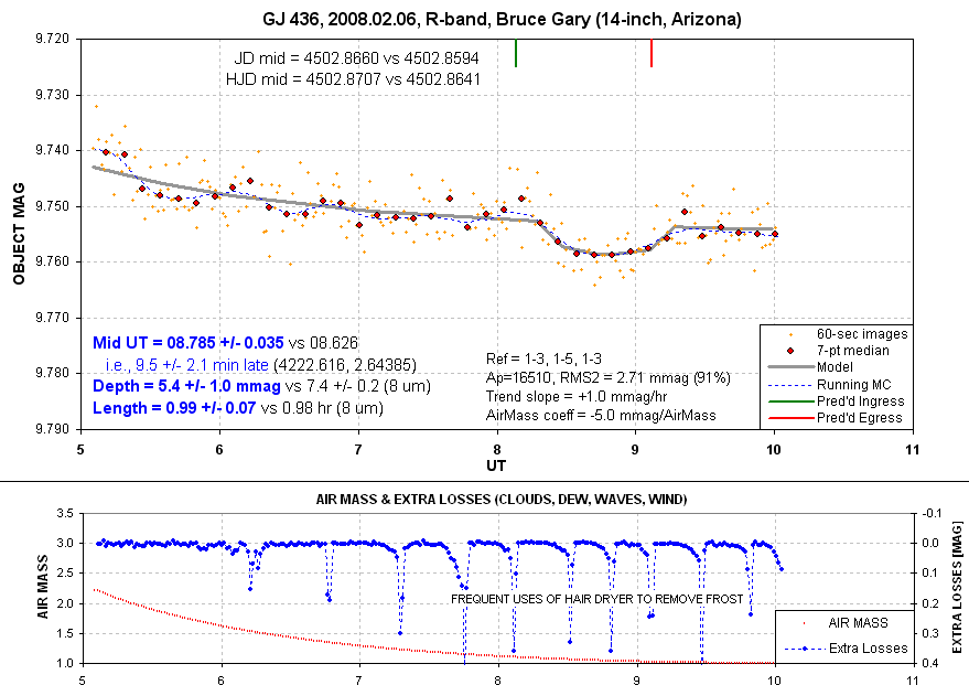
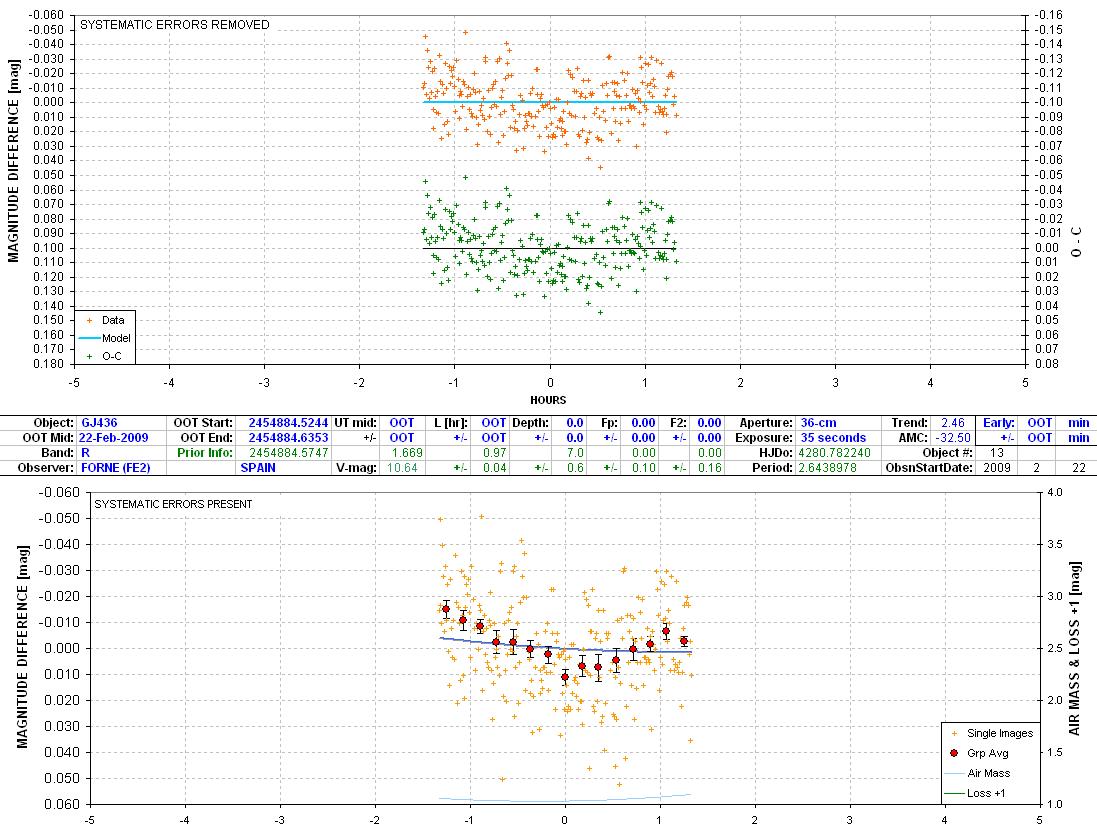
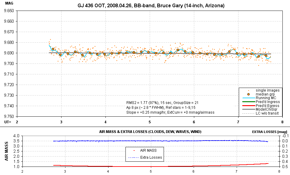
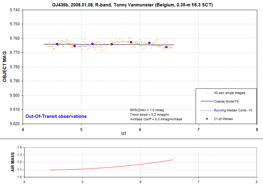
8206gary Frequent uses of a hair dryer to remove frost from the corrector plate; temp = 28 F, Dew Pt = 22 F (RH = 78%). WWV check of time tags.
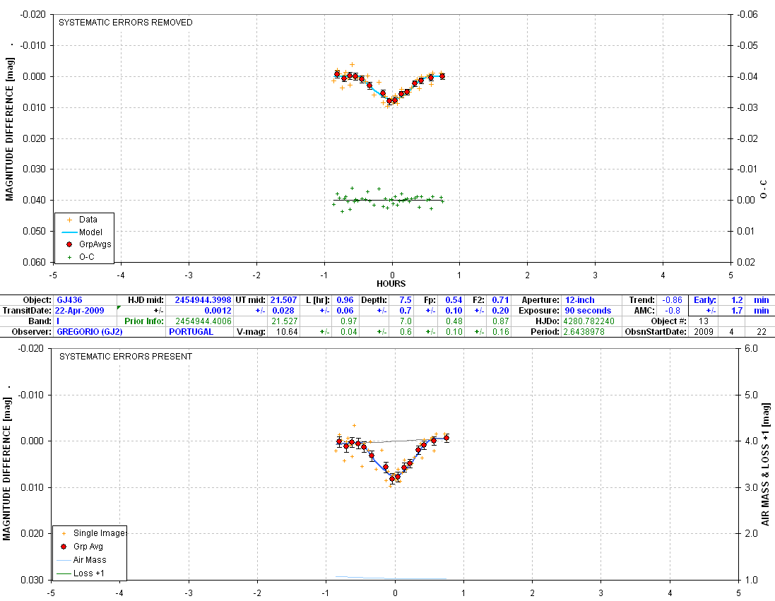
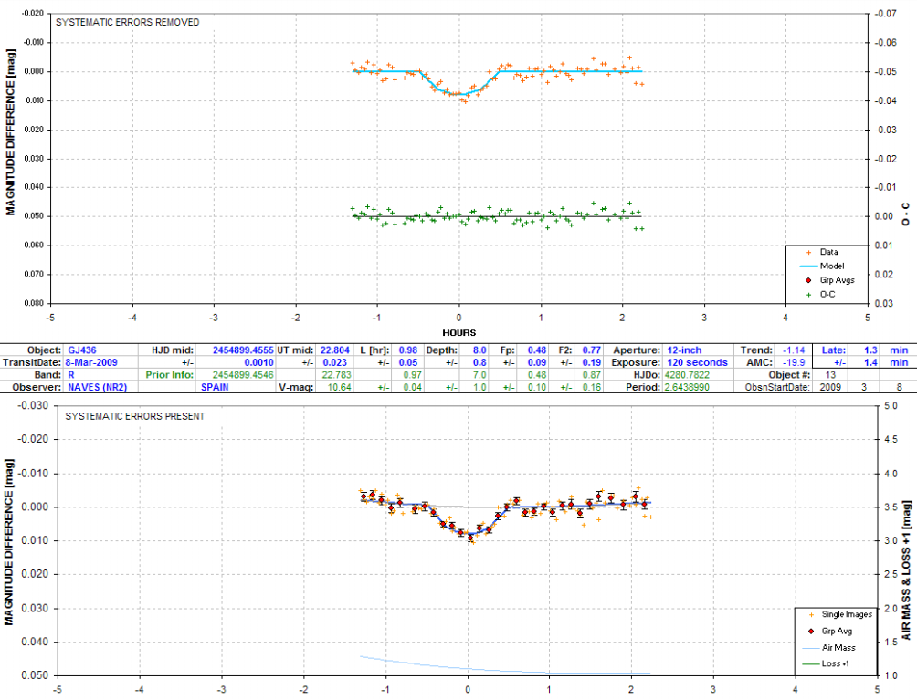
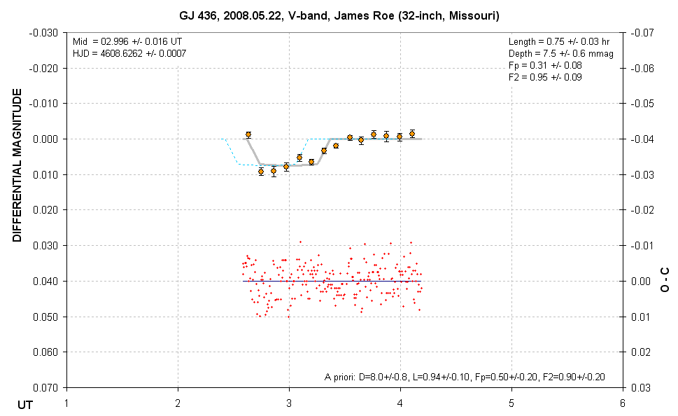
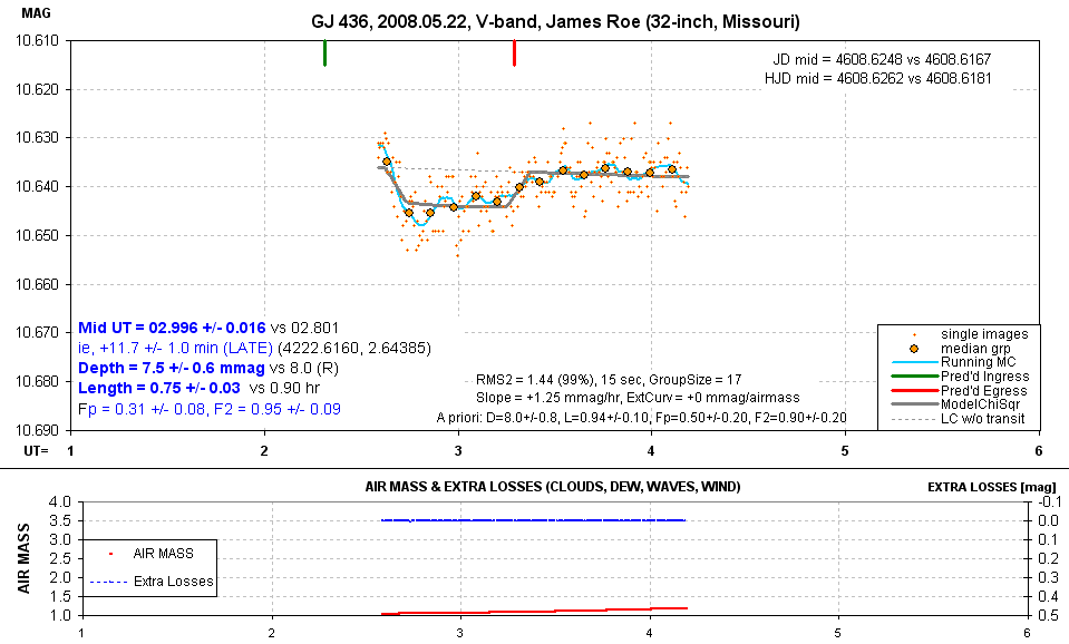
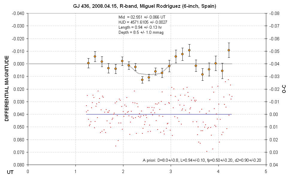
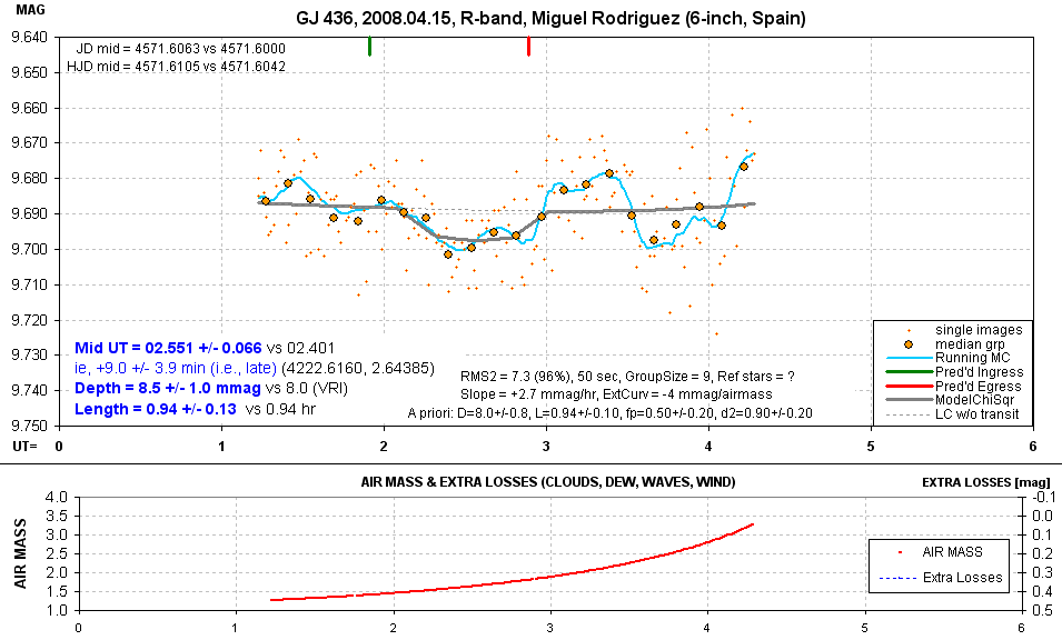
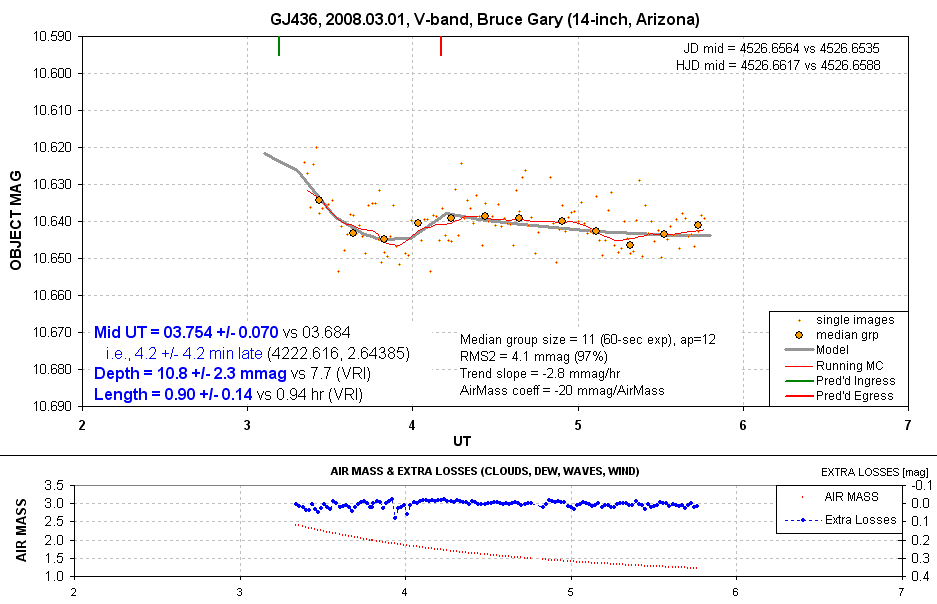
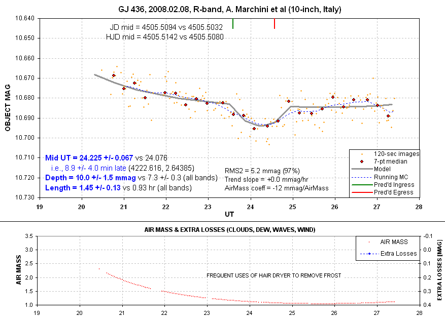
8206gary Frequent uses of a hair dryer to remove
frost from the corrector plate; temp = 28 F, Dew Pt
= 22 F (RH = 78%). WWV check of time tags.
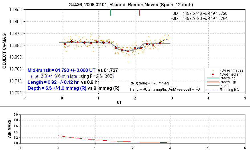
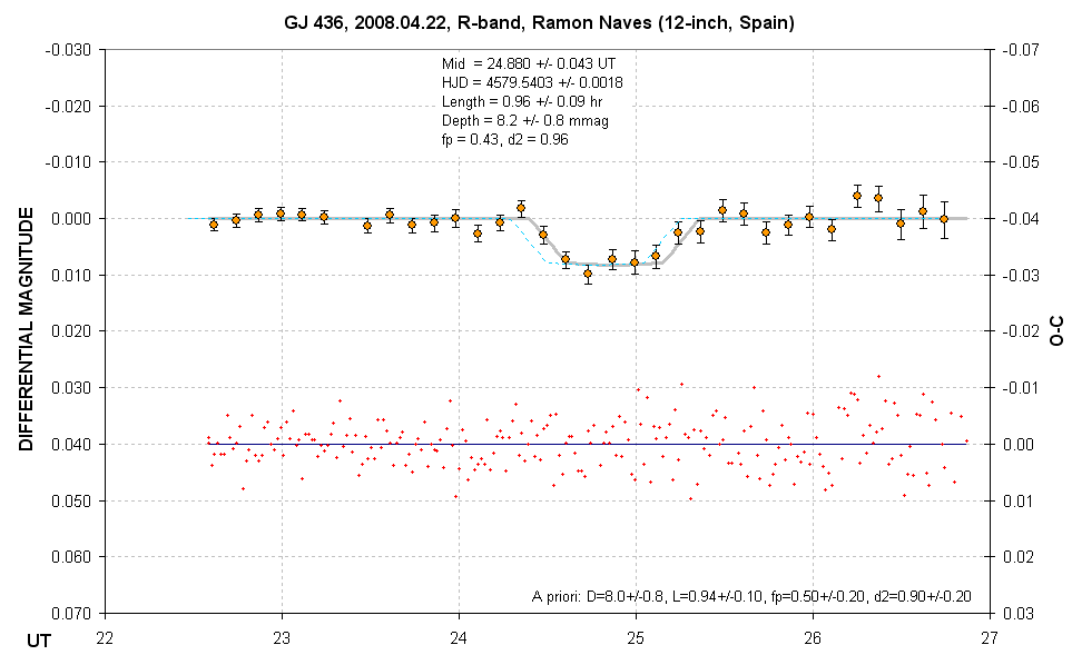
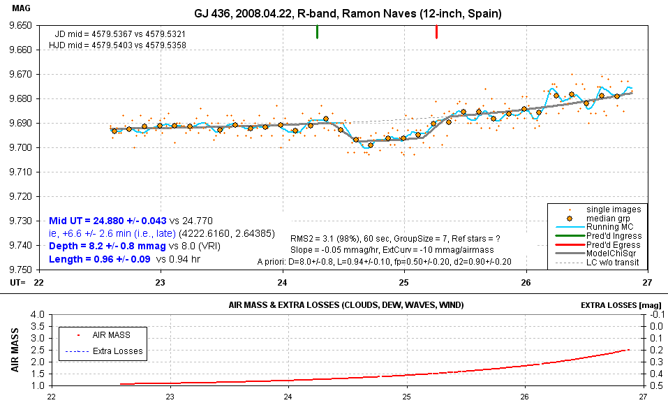
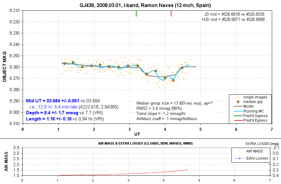
8201nave (waiting for permission)
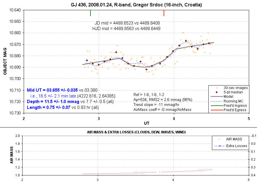
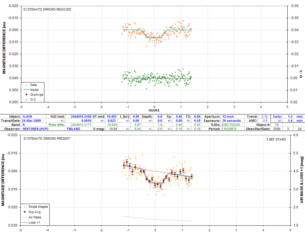
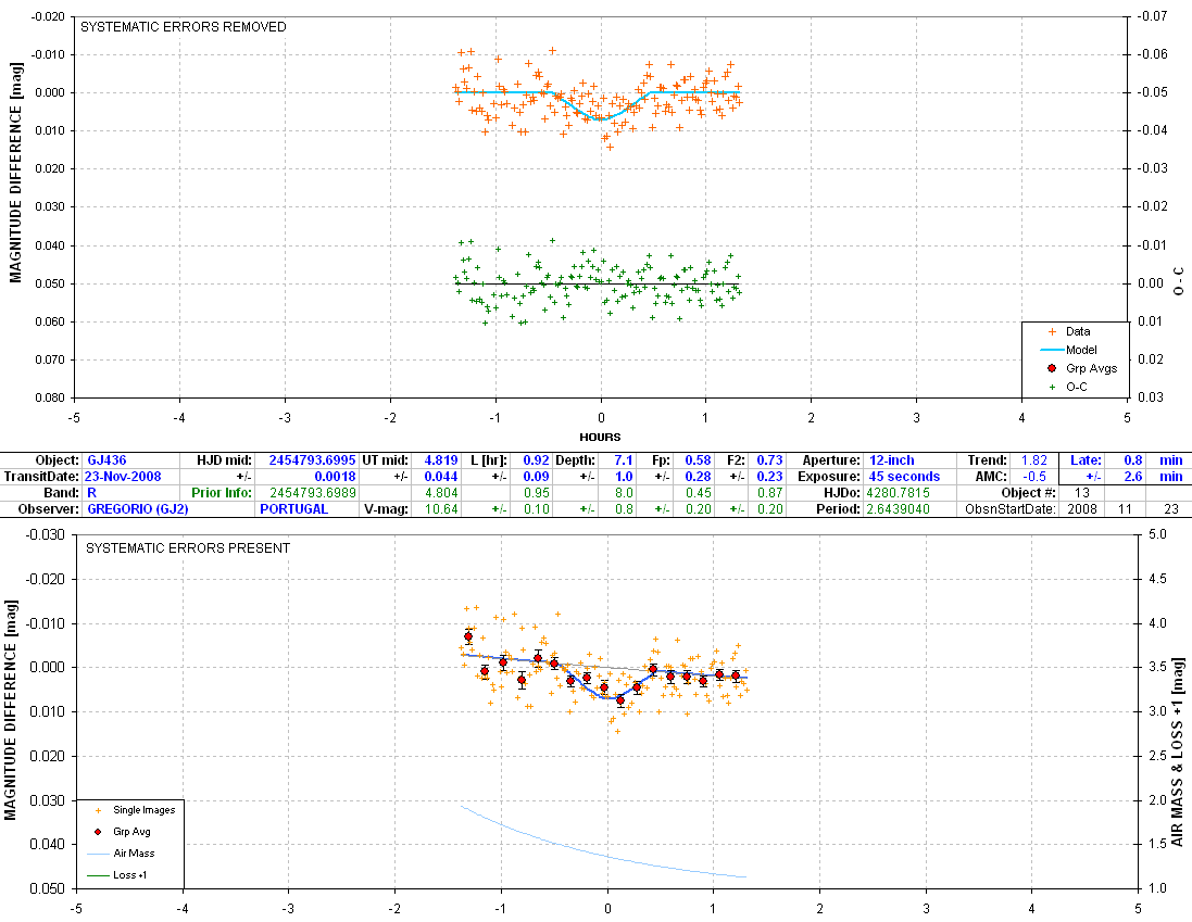
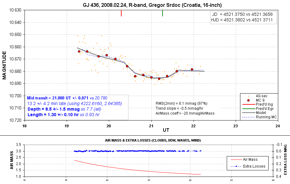
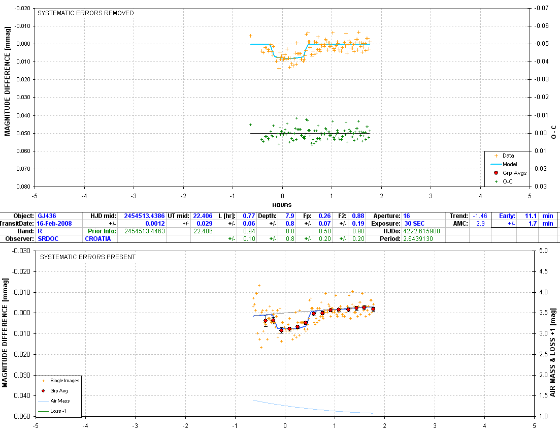
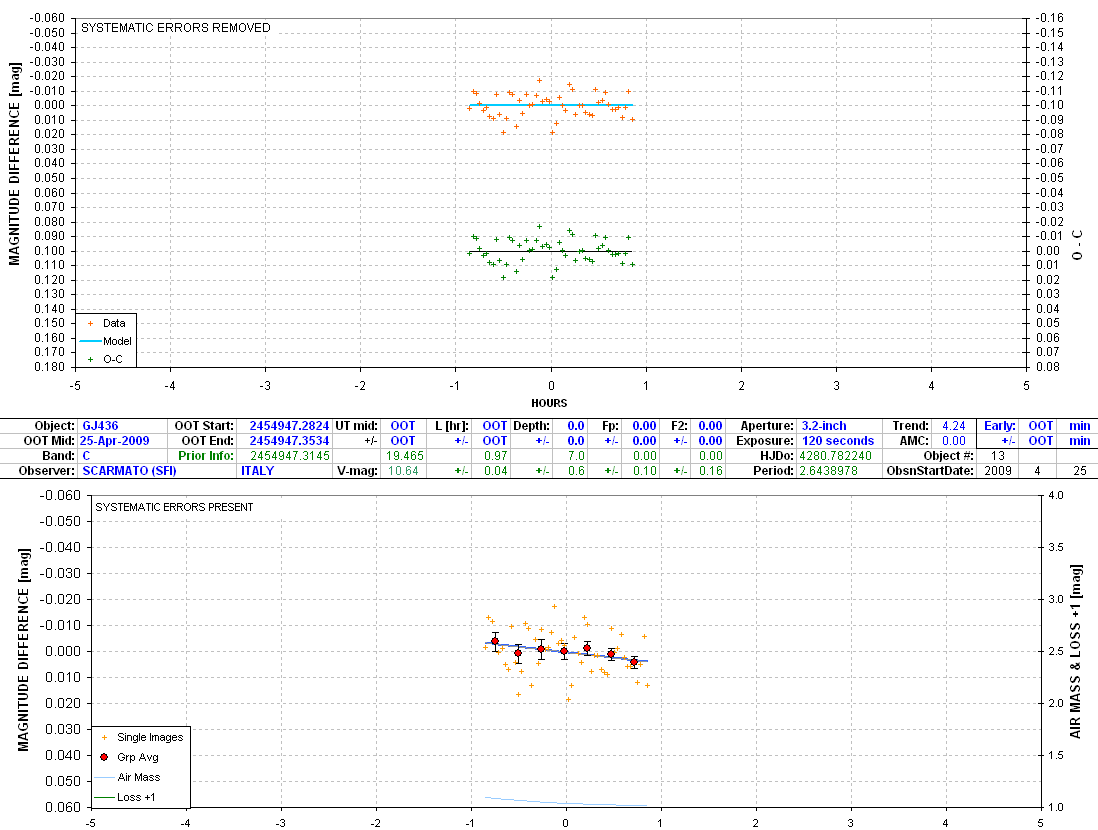
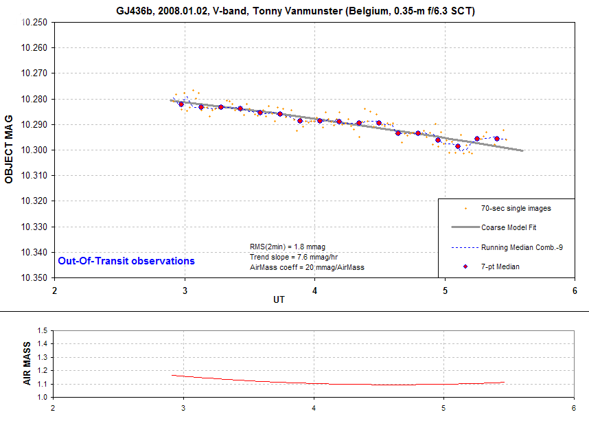
8124srdc The clock was checked & found to
be accurate.
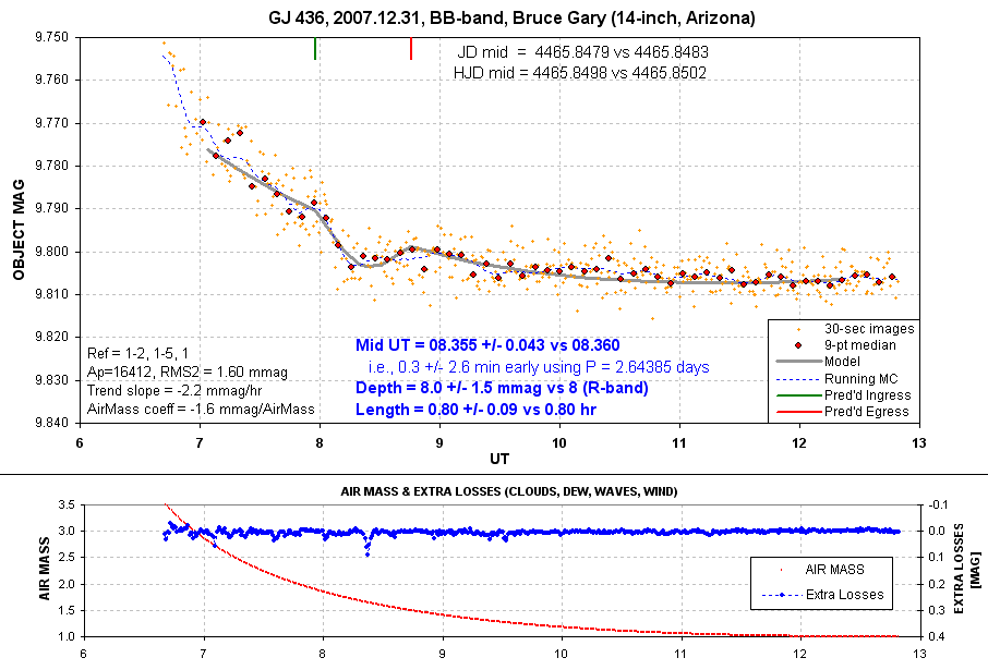
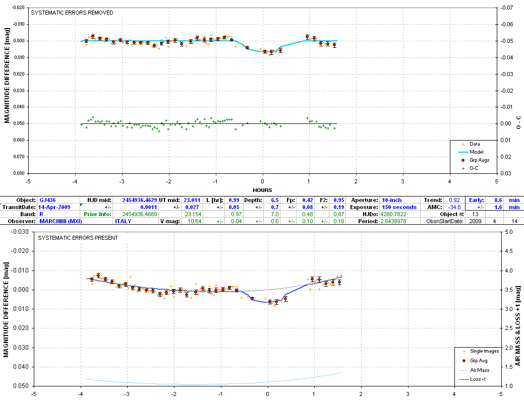
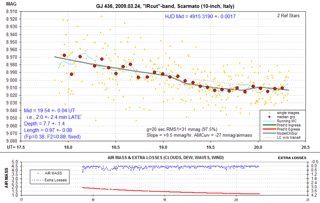
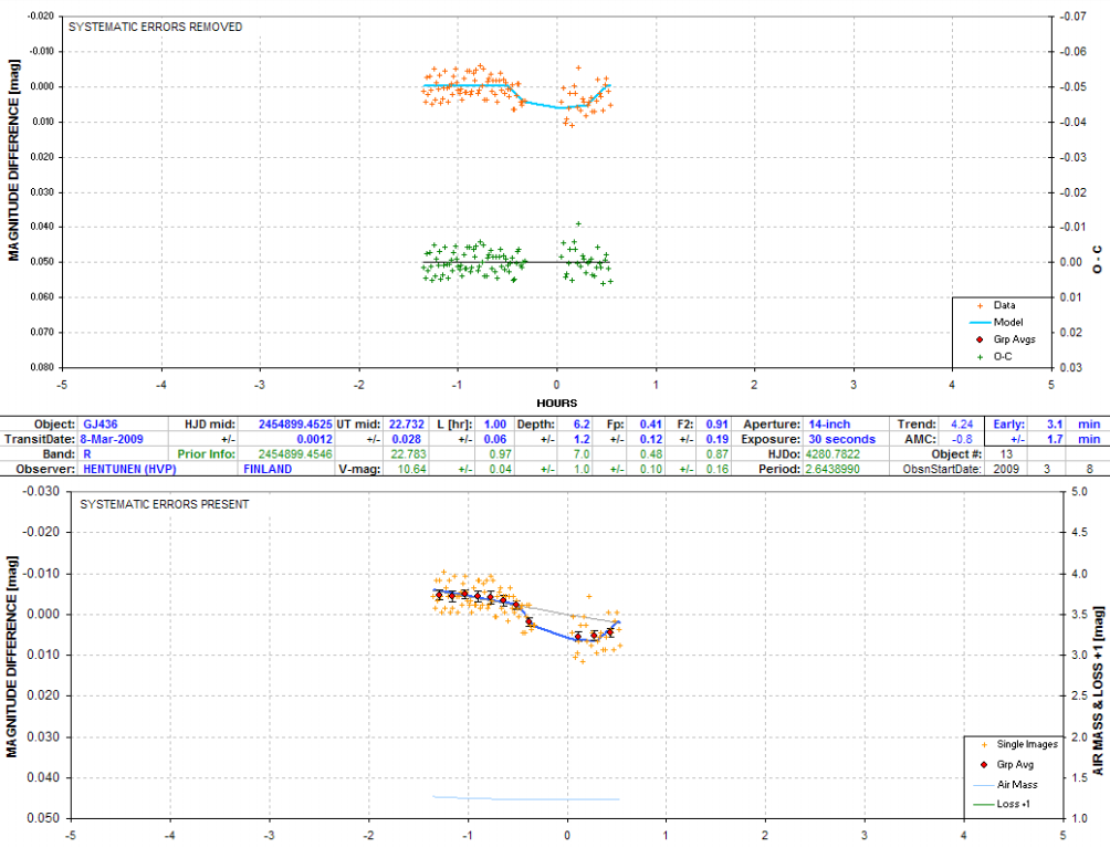
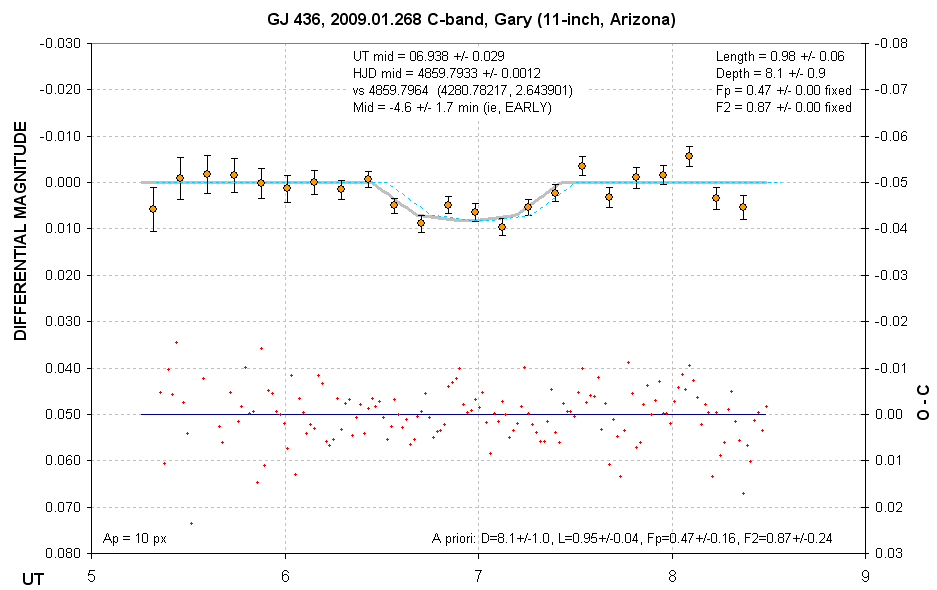
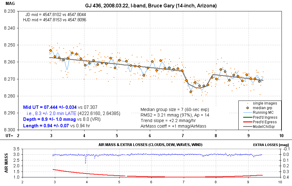
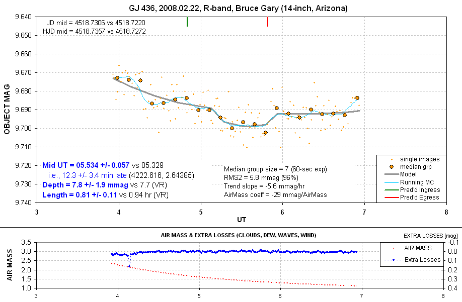
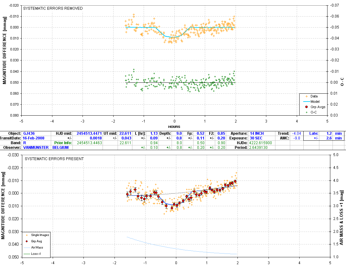
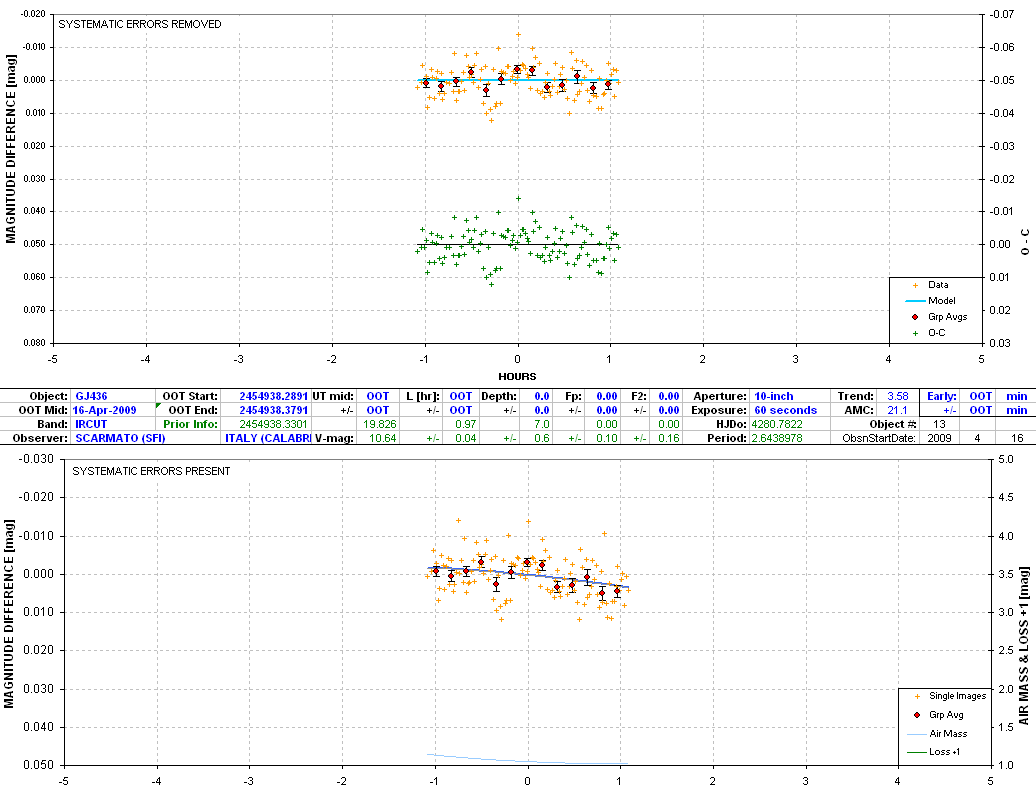
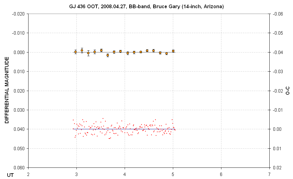
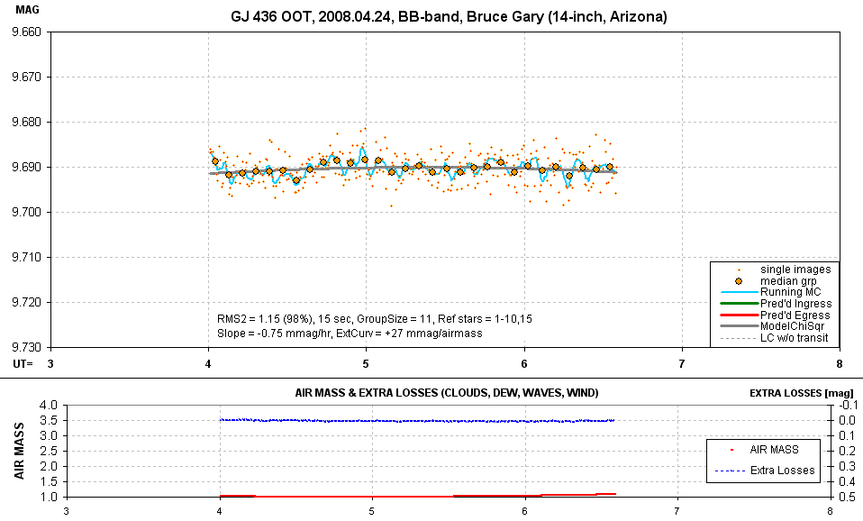
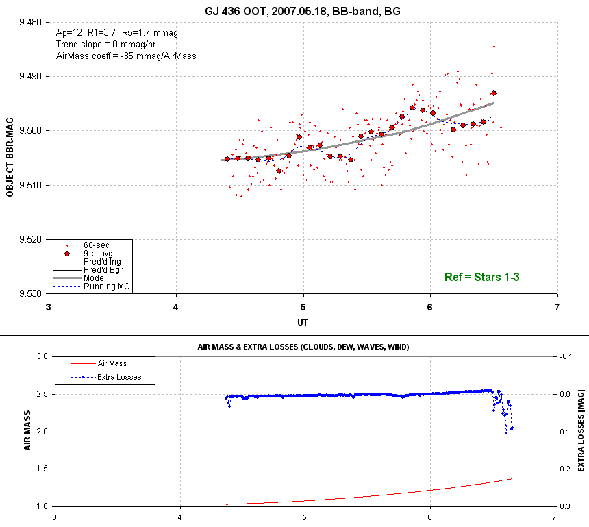
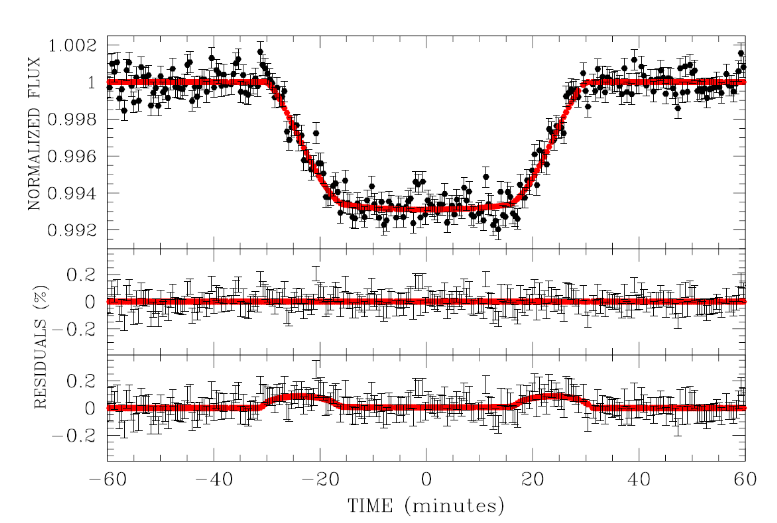
7c31gary Air mass curvature is high due to use
of a BB-filter and high air mass at the beginning.
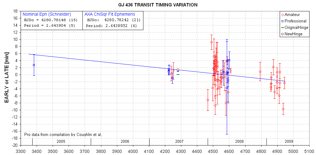
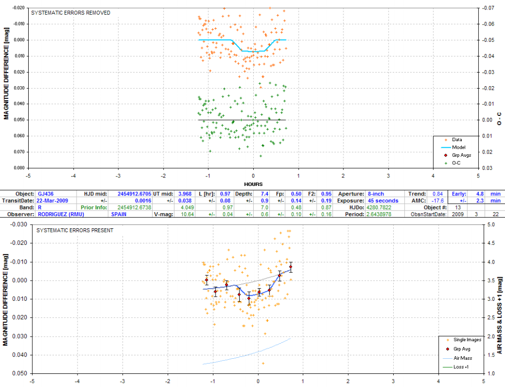
9222-13-FE2 OOT
The closest transit was at 23.06 UT on 2008.03.24
(i.e., 8.9 hrs before mid-observing session).
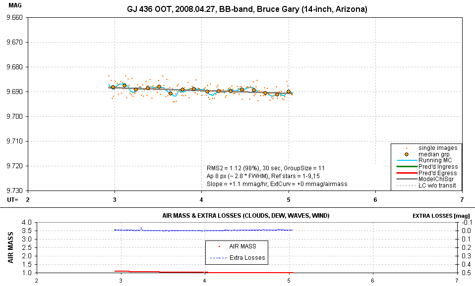
These observations were a test
of a new optical configuration which accounts for the
short duration. Nevertheless, there seems to be mild evidence
for 1 mmag variations on an hourly timescale.
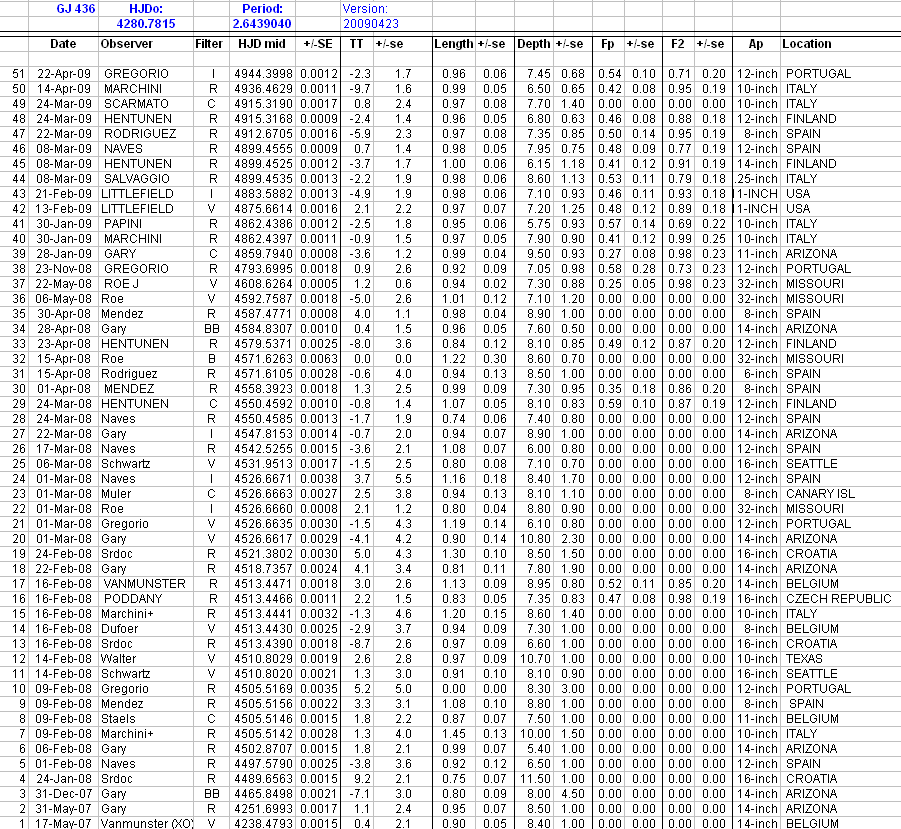
Professional Transit
Light Curves
Gillon
et al (2007) SST observations at 8 micron wavelength,
reproduced from Ribas et al (2008). Lowest panel shoes
effect of a hypothetical 0.1 degree inclination change
that could be produced by perturbations from a 5-Earth mass
outer orbit planet in a 2:1
resonant orbit.
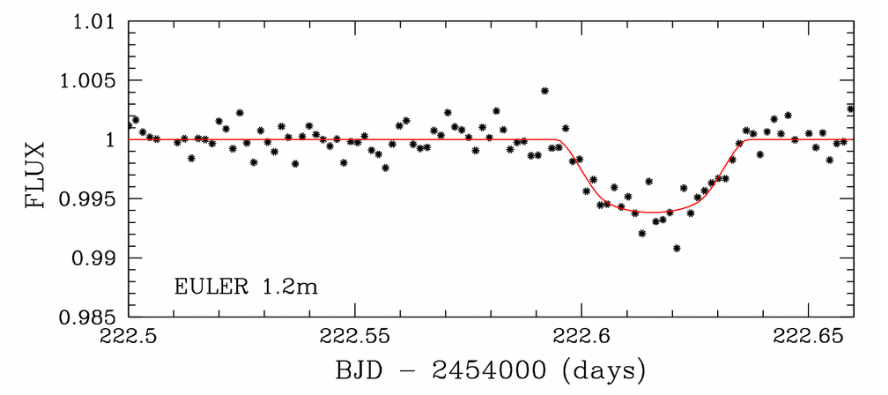
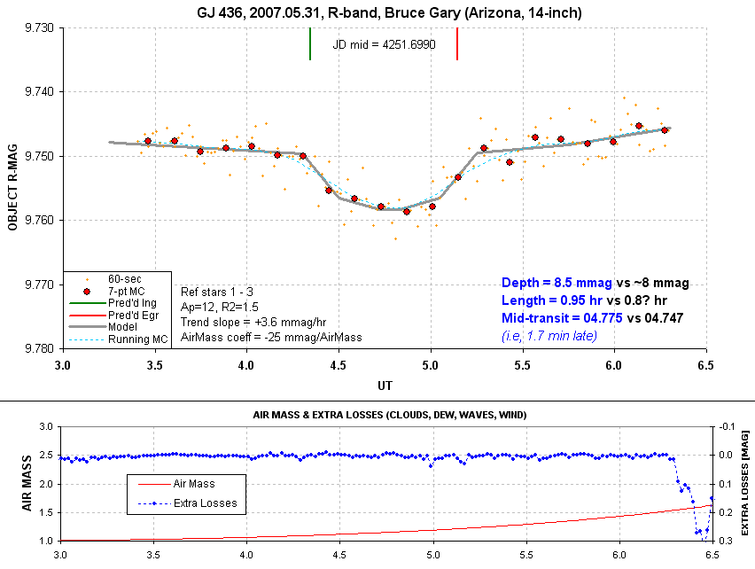
V-band,
Observatory of Geneva 1.2-meter Euler telescope at
La Silla Observatory, Chile (Gillon
et al, 2007). Mid-transit
at 2007 May 02, 02:41 UT. My measurements of this LC yield
depth ~6.5 ± 1.0 mag, length = 0.943 ± 0.064 hr.
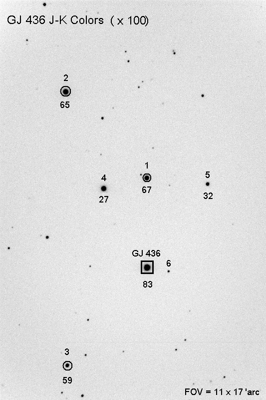
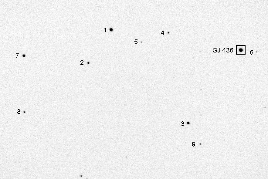
Figure F1.
Finder image with identifier star numbers (above)
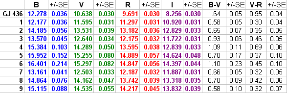
and J-K colors (times 100, below) selected stars. GJ 436 has
V = 10.68 and Rc = 9.66.
 .
.
Normally I don't present all-sky photometry results without completing
a second observing session and analysis and verify
compatibility between the two results. In this case
I have no plans for doing this since I doubt that anyone
will use any of these results.
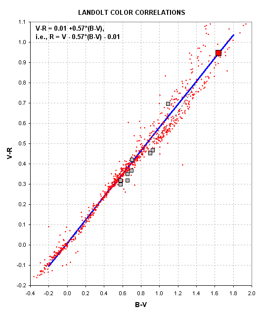
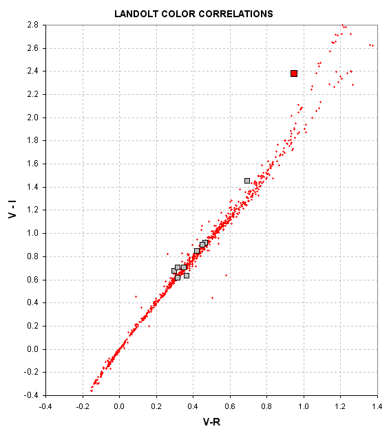
Figure A2 and A3. Color/color scatter diagram showing the location
of GJ 436 (red square) and the 9 nearby stars (gray
squares) in relation to 1259 landolt stars.
If the solution for one filter band had a systematic error it would show
up in these plots as a group offset in the color/color
scatter diagrams involving that filter. For example,
if all B-magnitudes were high by 0.05 magnitude then the
goup of gray squares and the red square would be offset to
the right by 0.05 magnitude. It's possible that such an offset
is present in Fig. A2, but it's clear that greater vaues fo such
an offset are very unlikely. An alternative for explaining the
rightward shift of Fig. A2 gray squares is for there to be instead
a downward shift, or values for V that are to negative by about the
same 0.05 magnitude amount. This is unlikely after inspecting Fig.
A3, where there is no evidence of shifts. Presumably, all 3 bands
(V, R and I) are free of calibration error offsets (unless by some
unlikely circumstance there are offset errors in all 3 bands that excatly
compensate to produce color/color agreement with the Landolot stars).
If it is true that V, R and I are free of calibration offset errors
greater than ~0.03 magnitude, then what should be make of the funny
location for GJ 436 in Fig. A3? I claim that it is inescapable that
GJ 436 has a much greater V-I color than the Landolt stars. Since V
appears to be normal (e.g., Fig. A2), we must conclude that I is anomalous.
In other words, these color/color scatter diagrams show that GJ 436
has an I-magnitude that is brighter than normal by ~0.5 magnitude!
I'll leave it to others to explain how this could be the case.
Note: It won't matter what magnitude you assume for reference stars for
the purpose of obtaining quality light curves. These
estimated values are presented for the purpose of
identifying star colors that "match" GJ 436's color which
can be useful in minimizing extinction related systematic
errors (i.e, LC curvature that's correlated with air mass).
In this table the column for R-band will be the most accurate
since it is based on observations. The other magnitudes for Stars
1 through 6 are based on JK magnitudes. For GJ 436 the B and I magnitudes
are based on color/color correlations for main sequence stars.
All stars in the table are compatible with main sequence color/color
relationships.
Gillon et al, 2007, Astron, & Astrophys., "Detection of Transits
of the Nearby Hot Neptune GJ 436" http://babbage.sissa.it/abs/0705.2219
Butler et al, 2004,
Astrophys. J. Lett.,"A Neptune-Mass Planet Orbiting
the Nearby M Dwarf GJ 436" http://adsabs.harvard.edu/abs/2004ApJ...617..580B
Ribas et al, 2008a,
Astrophys. J. Lett., "A ~5_earth Super Earth
Orbiting GJ 436?: The Poser of Near-Grazing Transits"
http://fr.arxiv.org/abs/0801.3230
Ribas et al, 2008b, IAU 253, Boston, MA, 2008
May 19-23
Alonso et al, 2008, "Limits to the planet candidate
GJ 436c" http://arxiv.org/abs/0804.3030
Bean et al, 2008, arXiv:0806.0851v2, http://arxiv.org/abs/0806.0851
Coughlin et al, 2008, preliminary
and final
(ApJL, pay)
Batygin et al, 2009, "A Quasi-Stationary Solution to Gleise 436b's Eccentricity,"
preprint: http://arxiv.org/abs/0904.3146
Return to calling web
page AXA
WebMaster: Bruce
L. Gary. Nothing on this web page is copyrighted. This site opened:
July 04, 2007. Last Update: 2009.08.02