ALL-SKY PHOTOMETRY
USING AMATEUR HARDWARE AND SOFTWARE
Bruce L. Gary (GBL) ; Hereford, AZ, USA
Abstract
This web page was started in the belief that all-sky photometry was
within reach of advanced amateurs with experience in differential photometry.
At the half-way point in its creation I have come to view it as a reference
for my use on some future date when I want to do another all-sky observing
session. I also include it on the web in case there's one other amateur motivated
to actually follow-through with the many tasks required for a proper all-sky
photometry analysis. The use of amateur hardware and software to achieve
0.020 magnitude accuracy for any of the BVRcIc filter bands comes with severe
handicaps, and I am reluctant to give encouragement that it should be attempted
by an amateur. It is best that some tasks be left to the professionals who
have access to software pipeline components with man-years of development
invested in them (e.g., star extraction using PSF-fitting). I apologize to
anyone who may feel encouraged by the existence of this web page to take
on the all-sky challenge if they encounter problems that seem to have no
solution. Don't blame me, I warned you!
Preface
Super-Simple
All-sky Photometry
Super-Simple Enhancements
Introduction
Fundamentals
and Terminology
Star Flux Equation
Considerations
Unique to All-sky
The Observing Session
Mid-Level Image
Analysis
Mid-Level
Spreadsheet Data Analysis
Iteration
for Star Color Solution
Final Magnitudes &
Finder Charts
Color-Color Scatter
Diagram
Upper-Level Image
Analysis
Upper-Level
Spreadsheet Analysis
Deriving V
and Rc from r' and JK
Appendix A: PSF shape effects
A Landolt star with V-mag = 8.61 is measured
to have a flux of 264765 counts near transit. The unknown target star "0607"
at the same elevation is measured to have a flux of 38767 counts. The brightness
ratio is 6.83, which corresponds to a magnitude difference of 2.09. The unknown
star is fainter, so it must have V-mag = 10.70. What's so difficult about
all-sky photometry?
|
PREFACE
The above example is based on two actual images, chosen without knowing
the result, which is off by only 0.03 mag. So, what is so
difficult about all-sky photometry?
I have identified 3 levels of sophistication in the procedure for performing
an all-sky photometry calibration of an unknown star field. The next section
contains the super-simplest method. Later sections include background material
on concepts, terminology, etc, which are needed for the more complicated procedures.
For the super-simple procedure all observations must be at the same elevation
angle, only the brightest Landolt stars can be used and its performace is
marginally acceptable only for V-band (where star color is least important).
The other two procedures can be used for calibrating star fields at more
than one elevation. The only difference between the second and third level
is speed and a slight improvement in accuracy; the third level is faster
but requires more facility with spreadsheets.
I have many web pages related to all-sky photometry. Here are some:
All-sky
phtotometry basic concepts (most are briefly included on this web page)
Photometry
for Dummies (list of several quick alternatives to the procedures on this
web page)
Photometry
for Smarties (an alternative to this web page)
Artificial
Star Photometry (emphasis on merits of using an artificial star)
SUPER-SIMPLE ALL-SKY PHOTOMTRY
This section may seem long to you, belying the name "super-simple," but
keep in mind that it's the same procedure in the box above with some averaging.
Let's assume you've already taken a set of V-band images of a Landolt star
field near transit and a set of V-band images of the unknown star field at
the same elevation. I'll use images from my 2008.01.19 all-sky observations
to illustrate this super-simple procedure.
1) Calibrate (dark and flat) the set of images (~7) of the Landolt star
field L0652 (at RA 06:52).
2) Median combine the L0652 images, calling this image L0652_MC.
3) From TheSky/Six read Landolt V-mags for the brightest stars.
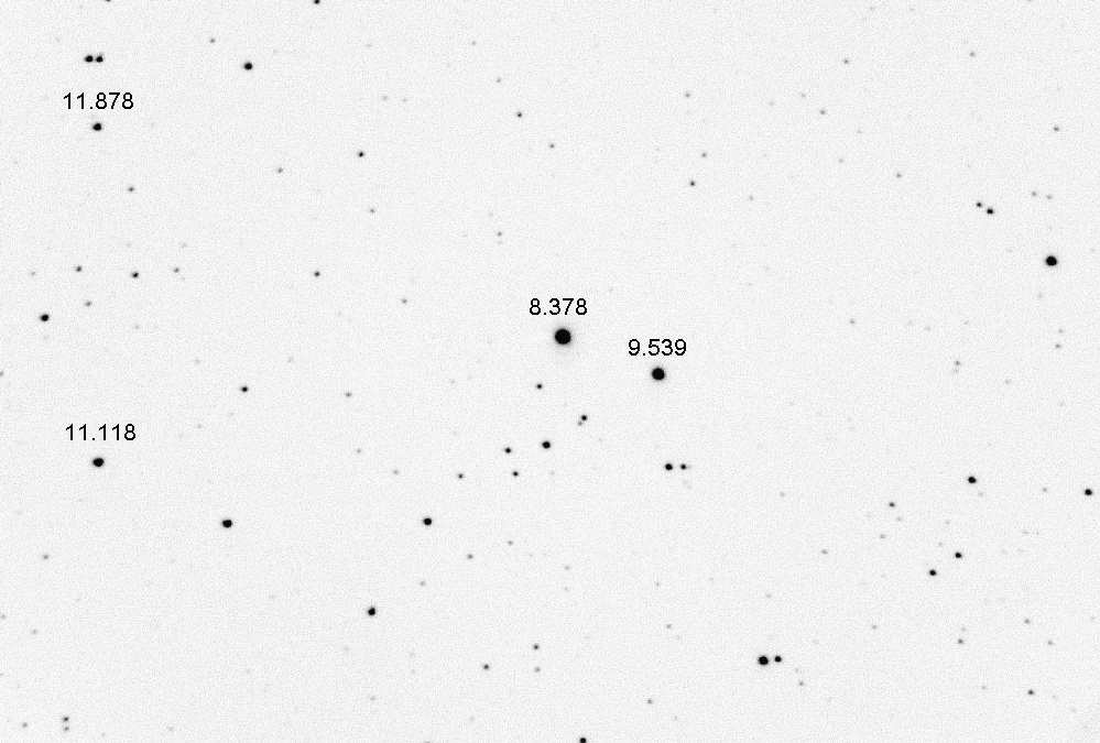
Figure 1. Landolt star field (L0652) showing V-mags for
brightest stars. FOV = 16 x 11 'arc, north up, east left.
4) Determine the FWHM of a bright star. For this example, it's 5.5 pixels.
5) Set the photometry aperture radius to 4 times FWHM, e.g. 22 pixels.
6) Measure the star fluxes ("intensities") and enter them in a table (or
spreadsheet) along with their V-mag values.
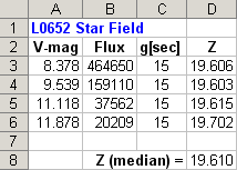
Figure 2. V-mag & flux readings for brightest stars in L0652.
Exposure time , g [sec], and a calculated parameter called "Z" are also shown.
7) Create a column for exposure time, g[sec]. Calculate a parameter called
"Z" defined as:
Z = V-mag + 2.5 × LOG (Flux [counts]
/ g [sec])
(Eqn. 1)
8) Median combine the several Z values. This is the telescope system's
Z-value for the filter and air mass for this one night (and maybe others).
9) Calibrate and median combine the "unknown" star field images, which
I'll call 2190_MC.
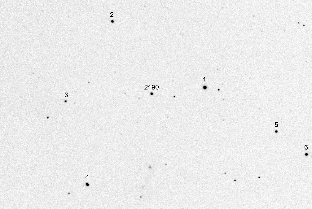
Figure 3. Unknown star field showing target "2190" and a few numbered
nearby stars.
10) Measure the flux of the target star, "2190", using a photometry radius
4 times the star's FWHM. For this example I meaure Flux = 14303 counts.
11) Calculate the target star's V-mag using the equation:
V-mag = Z - 2.5 × LOG (Flux [counts]
/ g [sec])
(Eqn 2)
For this example, V-mag = 12.16.
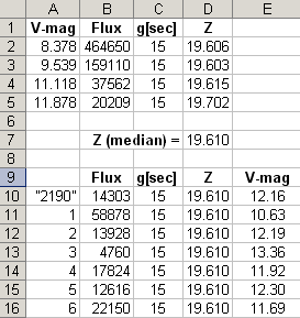
Figure 4. Calculation of V-mags for target and nearby stars.
The same equation can be used to convert fluxes for the nearby stars to
V-mags, as shown in the above spreadsheet.
This completes the description of the Super-Simple procedure for all-sky
photometry. Keep in mind that it is to be used for only those occasions when
all observations are at the same elevation (i.e., air mass). Also keep in
mind that this procedure works best for V-band (and maybe I-band), where star
color effects are minimum.
How did we do with this example? My final result for "2190" has V-mag =
12.135. The difference of 0.025 mag is better than typical for the uncertainty
that can be expected using this simple procedure; 0.040 mag is probably more
typical. The next section describes two enhancements that can be applied to
the super-simple procedure, which probably will produce V-mag accuracy of
~0.030 mag. The rest of this web page shows how to reduce this uncertaintly
to ~0.025 mag for V-band and the other bands, without the requirement that
all observations must be at the same air mass; the more sophisticated procedures
can also be used for observations using B, V, R and I filters.
SUPER-SIMPLE ENHANCEMENTS
Before proceeding with a proper introduction to the concepts and terminology
needed for an understanding of all-sky photometry as it is usually performed,
I want to call your attention to two shortcomings of the Super-Simple procedure
and ways to overcome them.
First, when we median combined images there was a small "scale change"
that depended on the order in which the images were combined. This is a subtle
effect, amounting to ~0.02 mag, typically, but as much as 0.04 mag on occasion.
The second effect has to do with star color. Every telescope system response
versus wavelength, for each filter, departs somewhat from the standard response
for B, V, Rc and Ic band shapes. This means that two stars having the same
V-band magnitude may produce slightly different fluxes for a real-world telescope
observing system. The size of this effect for V-band is typically 0.03 magnitude;
it's greater for R-mag, and much greater for B-band.
The "median combine scale change," leading to the correction that I'll
refer to as MC-cor, can be measured by comparing "median combine" image fluxes
with those from an "average combine" image. I'll refer to the "average combine"
of the 7 original L0652 images as L0652_MC. Any image that's the average combine
of several original images will be referred to as an AV-image. Average combining
won't change the scale, regardless of the order of the combining, and an
average combine is what the individual images "aspire" to represent. The
only problem with an average combine is that bad pixels, and cosmic ray defects,
just keep appearing as more images are combined. The median combine, on the
other hand, just keeps getting "cleaner" the more images are combined. There's
a way to have the best of both, and it consists of comparing fluxes (or magnitudes)
of bright stars from each image type. This is described next.
MC-cor is a ratio for multiplying MC fluxes to arrive at fluxes that would
be obtained from measurements of an image that is the average of several "clean"
images. A clean image is one withoutcosmic ray artifacts or pixel defects
(e.g., hot or cold pixels, usually produced by an imperfect master dark frame).
Suppose we have 5 bright stars (e.g., SNR > 300) in each of the AV and
MC images. For each star measure the magnitude in the AV-image and the MC-image,
and record the difference. Be sure to record "Mag_AV" minus "Mag_MC." Since
we're only dealing with magnitude differences it doesn't matter if the magnitude
scale is calibrated. Now, calculate the median value for this list of magnitude
differences, and call it "MC-cor Magnitude." Convert this to a ratio, MC-cor,
using the following equation:
MC-cor = 2.512 - MC-cor Magnitude
(Eqn. 3)
"MC-cor" is a multiplier adjustment. In other words the way we'll use it
is to multiply MC fluxes by MC-cor to arrive at fluxes that should approximate
what would have been measured from the AV image if all the original images
had been "clean."
For the L0652 images I obtained a list of "Mag_AV - Mag_MC" measurements
(for a series of bright stars) to be -4, -3, +1, -4 mmag, which has a median
of -3 mmag. Converting to a ratio we get MC-cor = 1.0028. For this case the
MC-cor correction is small, but let's incorporate it in this enhanced analysis
section.
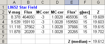
Figure 5. Incorporation of MC-cor, as a mmag version (column
C) and fractional correction (column D). The corrected Flux is Flux' (column
E). The new Z values lead to a new "Z (median)."
Star color is usually defined as B-V, or V-R. I use C = V-R - 0.37.
For a large number of main sequence stars the median V-R star color is +0.37,
so using my definition for C it will have a median value of zero on average.
There are many advantages to using this version, and they are treated later
in this web page. Since some Landolt stars have only B and V entries, it's
useful to have an equivalent version of C based only on B-V. This can be done
since main sequence star exhibit a good correlation between B-V and V-R colors,
namely: V-R = 0.57× (B-V). So, an alternative definition cor C is:
C = 0.57 × (B-V) - 0.37. I've adopted the convention
of giving preference to C = V-R - 0.37. This is summarized:
C = V-R - 0.37
if R-mag
is available
C = 0.57 × (B-V) - 0.37
if only B- and V-mags are available
(Eqns. 4a and 4b)
The tabulation of Landolt star magnitudes in the previous two figures can
be augmented with B-mag and R-mag, that are available from the Landolt database.
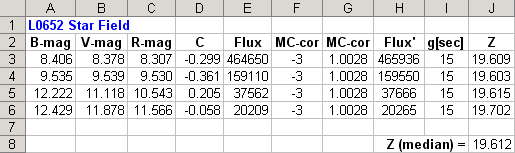
Figure 5. Enhanced version of an earlier figure, including
B- and R-mag, and a calculation of star color, C.
There's a large range of star colors in this list. Notice that the last
star's Z value appears to be an "outlier." This is due to the presence of
a nearby star within the signal aperture (almost discernible in Fig. 1). This
illustrates the merit of using median instead of average for adopting a Z
value. Here's the spreadsheet augmented to show V-mag calculated using the
adopted Z value of 19.612 and Eqn. 4a.
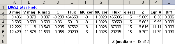
Figure 6. V-mag based on an equation (column K) and its
difference from Landolt V-mag (column L).
Does the equation V-mag differ from Landolt V-mag in a way that's related
to star color?
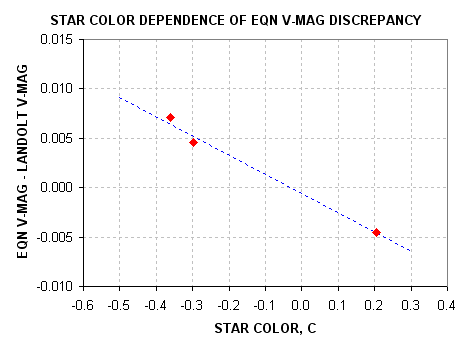
Figure 7. Star color dependence of equation V-mag discrepancy
with Landolt V-mag.
Yes, there's a pattern that requires that we brighten blue stars and fade
red stars in order to achieve agreement with Landolt V-mags. The V-mag discrepancy
has the equation dV-mag = -0.020 × C. We can therefore modify the equation
for calculating V-mag to be:
V-mag = 19.612 - 2.5 × LOG (Flux' [counts]
/ g [sec]) + 0.020 × C
(Eqn. 5)
This illustrates a method for enhancing the quality of star magnitudes
determined from the super-simple photometry algorithm described in the previous
section.
If we knew the target star's color we could enter a vlaue for it in the
above equation and derive a better magnitude. We should also determine an
MC-cor for the target star field and adjust the target star's flux accordingly.
Let's do these things.
For the "2190" star field I use some bright stars to measure MC-cor = "Mag_AV
- Mag_MC" to be -8, 0, +4, -1, +12, yielding a median MC-cor = 0 mmag. Star
color can be approximately determined from its 2MASS J and K magnitudes. J
= 10.345 and K = 10.774. Using Warner's JK to BVRI conversion equations yields
B = 12.84, V = 12.12, R = 11.72 and I = 11.33. The V-R color is 0.40, so
C = +0.03, which is very close to a typical star's color of C = 0. The following
spreadsheet incorporates the MC-cor and star color corrections.
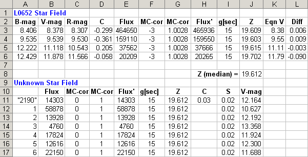
Figure 8. Final enhanced super-simple spreadsheet showing a revised
V-mag for "2190" that is based on MC-cor and star color estimated from 2MASS
JK magnitudes. "S" (column I) is star color sensitivity (c.f., Eqn.
5).
If I were to suggest a third enhancement of the super-simple photometry
algorithm it would be to repeat the above for R-band, then iterate star color.
But doing this involves an effort comparable to using a more sophisticated
all-sky procedure, so this is a good time to end the super-simple treatment
and begin some background that will prepare us for the mid-level and high-level
all-sky procedures.
INTRODUCTION
Sometimes I wonder if I'm making a thing too complicated. I worry about
star colors, differences in air mass, photometry aperture sizes, etc. Am I
worrying about these things because they're necessary for achieving accurate
magnitudes, or because I enjoy the process of figuring out how these things
can affect the measurement? I'll let the reader judge this after working to
figure out this web page.
If the earth didn't have an atmosphere that absorbs starlight then all-sky
photometry would be trivial. The observer would merely take a CCD image of
a region with well-calibrated stars, then another image of the region of interest
with the same settings. If the spectral response function of the telescope/filter/CCD
system for the filter band closely resembled the standard spectral response
for the corresponding BVRcIc bands then no additional corrections would be
needed. To the extent that the system spectral response differs from the
standard one, small corrections related to star color would be required. The
"CCD transformation equation" corrections for this high-quality space-borne
system would be straightforward given that they would depend on only star
color (not atmospheric extinction).
For the observer on the Earth's surface, using a telescope system with
an imperfect spectral response, more things have to be done. The atmosphere
absorbs different fractions of a star's light at different elevation angles
(air masses). A star's color as it enters the telescope aperture will depend
on how much atmospheric absorption has occurred (since atmospheric extinction
depends on wavelength). Seeing causes the point-spread-function (PSF) of
the star to be broad, and not necessarily circularly symmetric; imperfect
tracking also contributes to the broadening of the PSF in a preferential direction
and will be different from image to image. This last problem means that a
photometry aperture may not capture the entire flux from the star, and the
flux recovery fraction can vary from image to image. This and other real-world
problems means that additional analyses are required to make a proper measurement
of an unknown star's magnitude based on measurements of standard star fields,
and this extra analysis can sometimes take an enormous amount of labor (unless
all matters are dealt with by a pipline of programs). Nevertheless, these
things can be done by an amateur, but the amateur must be devoted to the
task.
My teaching philosophy is to describe a concept, then give a specific example
with real data that illustrates the concept. I've gradually learned that some
people don't care for concepts, and would rather be presented with a cookbook
procedure to follow. I'm assuming that you're not one of those people.
Another of my teaching philosophies could be described as "approaching
a problem with successive approximations." Second-order effects just get
"in the way" when the first-order effect is being learned.
Since I've created many web pages describing all-sky photometry I'll include
links to those web sites at appropriate times.
The first three sections of this web page may be tedious, and it will be
OK for the reader to skip past them while keeping in mind that they can be
referred to if a concept or term is unfamiliar.
Finally, since I've figured out just about everything I know by floundering
alone, and referring to a book or internet only when I'm stumped, my procedures
for doing some things are unconventional. As any programmer knows, there's
no such thing as "the correct" program code; any program that yields the right
answers is "correct." My concept-driven procedures for all-sky photometry
yield the right answers, as I've demonstrated, but don't be surprised if you
compare what I do with what someone else does and you find procedure differences.
A relevant example of this is the use by most professional astronomers, and
the recommendation by the AAVSO, of "CCD transformation equations" for transferring
magnitudes from standard stars in an image to an unknown star in the same
image (i.e., differential photometry). When I studied this procedure I was
appalled by how unecessarily complicated it was, and by how error prone it
was because it was non-intuitive. It seemed designed for use with mechanical
calculators, or maybe logarithms, which in fact it was. I gleaned the concepts,
derived those CCD transformation equations from first principles, then proceeded
to create an entirely new procedure that lends itself to use by personal computers
with spreadsheets. If you want to see that old fashioned, cumbersome approach,
then click on CCD transformation
equations derived. If you want a concept-driven approach, then keep reading.
Here's a list of some of my all-sky related web pages:
Photometry
for Dummies A summary of options, from simple to complicated, for assessing
a star's BVRI magnitudes with various accuracy goals
Photometry
for Smarties A summary of conepts and procedures I developed for
all-sky photometry, that is a little out-of-date (this page will be better)
All-Sky
Photometry Concepts A slower-paced description of background material,
some of which appears here
Artificial
Star Photometry A brief description of why an artificial star is
a useful tool for assesing what's going on with funny-looking data
Please give me feedback on what isn't explained well.
FUNDAMENTALS AND TERMINOLOGY
It's not absolutely necessary for you to read this section now since you
can refer to it when you encounter a puzzling term in later sections. I like
having a terminology section near the top of a document. I'll use this section
to also cover, very briefly, some fundamental concepts associated with the
terminology. A fuller version of most of the material in this section can
be found at All-Sky Photometry
Concepts.
When photons from a star are absorbed by the silicon crystal in a CCD chip
there's a good probability each photon will release one "photoelectron." The
probability of this depends on wavelength (quantum efficiency). When the
CCD is "read" the photoelectrons from a specific pixel on the CCD are summed
and converted to a number, or ADU (analog-to-digital unit). The sum of ADU
counts on neighboring pixels associated with a specific star is called the
star's "flux" - usually abbreviated by the letter S (MaxIm DL uses the term
"intensity" in place of flux). A star's flux reading will be proportional
to the star's "brightness" and also the exposure time. I use "g" to represent
exposure time (engineers use the term "gate time" to represent the interval
between the start of counting v/f converter output pulses and the ending time).
Recall that magnitude is defined by this equation: Mi
- Mo = 2.5 * LOG10 (S0 / Si
) where S0 is a known magnitude. Another way to write it is Si
/ So = 2.512(Mo - Mi) .
Atmospheric absorption is proportional the the number of molecules of air
and aerosol particles along the viewing direction's line-of-sight. Air mass,
m, is the ratio of the number of molecules and aerosols at in given
direction to what it is at zenith (assuming no horizontal gradients in anything).
I use the term "m" for air mass instead of "X" mostly because that's what's
done in the atmospheric sciences, where I worked before retirement. Since
absorption by each atmospheric layer removes photons from what's incident
upon it, the flux at ground level versus air mass m is given by S(m) = S(m=0)
* e(-m * tau), where "tau" is "optical depth" at zenith. Another
way to treat atmospheric extinction is to combine the two equations in the
previous paragraph and conclude that a star's apparent magnitude varies linearly
with air mass:
Mi - Mo = m × tau × [2.5 × LOG10 (e)].
The bracket term is the constant 1.0857. Note that magnitude changes linearly
with air mass, m, and the rate at which it changes with m is 1.0857 ×
tau, which is referred to as the atmosphere's "extinction coefficient" - which
I will abbreviate using the letter X. So, Mi = Mo + m × X.
Star color is usually referred to by differencing two magnitudes, such
as B-V. Star color can also make use of V-R, V-I and a J-K, for example.
I'm going to invent a new "star color" convention guided by the desire for
it to be zero for a typical star. The reasons for this will become obvious
later. For main sequence stars (90% of stars) the median B-V is 0.64 (actually,
this is really just the median of the 1259 Landolt stars). A good fit for
the relationship between B-V and V-R is:
V-R = 0.57 × (B-V)
is an approximate conversion between
V-R and B-V
(Eqn. 6)
Amateurs have small apertures, and it's chronically difficult for us to
measure star fields with a B-band filter. It often occurs that in performing
an all-sky phtometric solution for a star with unknown color the V-R magnitude
difference is well determined whereas the B-V magnitude difference isn't.
Therefore, I've found it useful to consider defining star color to be zero
for the median value of V-R. The median V-R is 0.57 × 0.64 = 0.37. So,
my star color is: C = V-R - 0.37, or the equivalent C =(B-V)/0.57 - 0.64.
For very red stars I've found it useful to invent a version of C that has
a closer-to-linear relationship with photometry observables: C' = C + 0.5
× C3, but don't worry about this now. To summarize these
star color conventions:
C = V-R - 0.37
when R is available
(Eqn. 7)
C = 0.57 × (B-V) - 0.37
when R is not available
(Eqn. 8)
C' = C + 0.5 × C3
(Eqn.9)
Another term I'll use is "flux recovery fraction," defined as the ratio
of flux measured by a photometry aperture to the flux that would be measured
by a very large photometry aperture. The two fluxes could easily differ by
several %, especially if the target star or some of the Landolt stars are
faint. We need to worry about any effect larger than ~0.5 % in order to achieve
our goal of absolute accuracy = 0.025 mag (2.5%) for V-band. Since the point-spread-function
(PSF) for most stars in a CCD image has a Gaussian shape it is possible to
express the ratio of fluxes as a function of the ratio of PSF half-width (FWHM)
and aperture radius. The ratio of aperture radius to FWHM is r = aperture
radius [px] / FWHM [px]. The ratio of fluxes is f(r), where f stands for
flux recovery fraction. The flux recovery fraction correction, f-cor,
can be expressed in terms of magnitude, and can have the form f-cor = 800
[mmag] / ( r 4 ).
STAR FLUX EQUATION
When the flux from a star in a CCD image is "measured" you're summing the
ADU counts (produced by photoelectrons) that are within the aperture "signal
circle." It will be useful to consider how this flux compares with a hypothetical
observing system in space that has a perfectly constructed spectral response
shape for the filter in use. Let's consider for a moment the flux rate, or
flux per unit of exposure time, S / g. If the hypothetical space-borne system
yields a flux rate of So / g, and we measure S / g. The two are
related by the following:
S / g = So / g ×
(constant related to apertures, dirt on optics, CCD's QE, etc)
× (fraction
surviving passage through atmosphere)
× (relative
response for star with its color)
× (flux recovery
fraction)
× (star color
change after passing through atmosphere and system's sensitivity to this)
(Eqn. 10)
The concepts in the above equation can also be expressed in terms of magnitudes,
which I refer to as the "flux to magnitude equation" and presented here (using
V-mag in this example):
V-mag = Zo - 2.5×LOG10 ( S / g ) -
m×X + S×C' + f-cor + H×m×C'
(Eqn. 11)
where Zo is a zero-shift constant (unique to the hardware in use), S is
measured flux, g is exposure time, m is air mass, X is zenith extinction
[mag/airmass], S is a star color sensitivity coefficient (unique to the hardware),
C' is the linearized star color (C + 1.3 × C2),
which in turn is based on star an un-linearized star color (C = V-R - 0.37
or C = B-V - 0.64), f-cor is a correction for the fact that S is not the
entire flux registered on the CCD from the star being measured using a possibly
small aperture, and H is coefficient correcting for the fact that star color
entering the telescope is different from star folor incident upon the atmosphere.
I find it convenient to convert S to Stotal within a spreadsheet
where I enter FWHM and photometry aperture. The last term is only important
for unfiltered observations (or blue-blocking filter observations), so it
can be dropped when performing observations with BVRcIc filters (which I'll
henceforth refer to BVRI). The above equation then simplifies somewhat to:
V-mag = Zo - 2.5×LOG10 ( Stotal
/ g ) - m×X + S×C'
(Eqn. 12)
My 14-inch telescope, for example, has the following V-mag equation:
V-mag = 19.76 - 2.5×LOG10 ( Stotal
/ g ) - m×0.16 [mag/airmass] - 0.02×C'
(Eqn. 13)
The Zo term is amazingly constant for months, but it changes with any configuration
change, such as introducing a focal reducer, or letting the cover plate become
dirty. The zenith extinction coefficient of 0.16 [mag/airmass] varies with
the seasons from ~0.15 to 0.19 [mag/airmass], and exhibits day-to-day changes
smaller than this variation. The star color coefficient, -0.01, remains constant
for months at a time, but will change when the hardware configuration changes.
All of the constants are different for the different filter bands.
Notice in this last equation that when the target star's color is not known
we can assign C' the value zero knowing that this is justified for stars with
a color similar to the median star color. For this case the above equations
implifies to:
V-mag = 19.76 - 2.5×LOG10 ( Stotal
/ g ) - m×0.16 [mag/airmass]
(Eqn. 14)
Landolt star fields are used to solve for the constants in the above equation.
It's a good practice to observe the Landolt star fields every night that an
unknown field of stars is to be calibrated. It's risky, but sometimes a necessary
expedient, to forego the Landolt star field observations on a particular
night and simply use the equations derived from previous sessions. Since
this risky strategy is so convenient (converting star flux to magnitude in
a matter of seconds, using only a hand calculator), I sometimes do it, knowing
that the answer could be off by 0.05 magnitude (because of an incorrect assumption
about extinction on the night in question, etc).
There's another simplification of the "flux to magnitude equation" that
can be made when the target star field is observed at the same approximate
air mass as the Landolt star field: the extinction term may be dropped but
the star color term should be retained. Thus, using my V-mag equation for
illustration:
V-mag = 19.76 - 2.5×LOG10 ( Stotal
/ g ) - 0.02×C'
(Eqn. 15)
This flux to magnitude equation can be used to evaluate the zero-shift
constant (19.76 in the above equation) using a set of Landolt stars, and if
the Landolt stars have a wide range of colors the last term's coefficient
value can also be checked. Since the target star field will be at the same
elevation angle (air mass) it's not necessary to include the extinction term;
if it's included it won't contribute anything, but there won't be an opportunity
for evaluating the zenith extinction coefficient for the observing session.
This is the form of the flux to magnitude equation that we'll use for the
"simple first observation."
CONSIDERATIONS UNIQUE
TO ALL-SKY
Everyone coming to the task of all-sky observing has many observing precautions
that were necessary for whatever previous observing tasks. For example, I
frequently complain about the unsuitability of German equatorial mounts (GEM)
for exoplanet observing because whenever there's a meridian flip during an
observing session it usually produces a discontinuity in the light curve with
a magnitude of a few mmag. For all-sky photometry, however, this is rarely
a problem, and in fact it can be turned to your advantage by observing the
same star field on both sides of the meridian flip. The goal for exoplanet
light curves calls for constancy of whatever systemtic errors are present,
to a few mmag level. Even if the size of the systematic error is large it
will be unimportant if is varies lineaerly with air mass (i.e., due to extinction)
or with time (i.e., due to star field movement through a flat field with low
spatial frequency errors). For all-sky observing errors of a few mmag is
unimportant since our goal is achieve accuracy of ~20 mmag to 30 mmag. An
error of 5 to 10 mmag will have negligible effect upon the the all-sky calibration,
even if these errors vary erratically.
Another difference between requirements for exoplanet light curve observing
and all-sky observing has to do with precision versus accuracy. Recall that
accuracy is all about reducing systemtic errors whereas precision is all about
reducing stochastic (Poisson) noise. Also, accuracy is the orthogonal sum
of calibration uncertainty and precision. Whereas exoplanet LCs require a
precision of 1 or 2 mmag, and any old accuracy that is present, all-sky observing
demands an accuracy of ~2%! Another way of stating this is that precision
SE and systematic calibration SE uncertainty must orthogonally add to nothing
greater than ~2%. Attaining a precision of <2% is easy for all but the
faintest Landolt stars (which aren't worth trying to use), so the entire
burden of achieving ~2% accuracy (20 mmag) rests with controlling calibration
uncertainty. Therefore, exposure times can be short since we only require
that SNR > 200 (e.g., 5 mmag). Note that if we're "fighting" 2% calibration
sytematics (~20 mmag) a 5 mmag stochastic SE added orthogonally yields 20.6
mmag accuracy SE.
Another issue that's important for all-sky observing but isn't important
for exoplanet LC observing is sky conditions. A "photometric sky" means there
are no clouds in sight and the wind is calm. Whereas exoplanet observing can
be continued in the presence of thin cirrus all-sky observing can be a total
loss in the presence of these clouds. The "calm wind" requirement is related
to the fact that any horizontal gradients in aerosol burden are carried through
the line of sight by wind, and this translates to high winds creating large
temporal changes in zenith extinction. When zenith extinction is changing
fast we cannot assume a constant extinction versus time, which means that
a Landolt calibration may not apply to a target star field image made at
a different time. Straddling the target images by Landolts before and after
reduces this problem.
Flat fields are very important for all-sky photometry; more important than
for exoplanet LCs. If you don't get good ones on the same night as the all-sky
observations, it's best to abandon the all-sky observing rather than waste
time on a flawed set of images. There's clarifiaction that should be made
about flat fields being only good for stars the same color as the sky light
entering the aperture. Whereas this is true, the fact that twilight is blue
doesn't invalidate these flat fields for all-sky photometry of red stars.
This is because one of the steps in all-sky image analysis is solving for
star color dependence on measured flux.
Focus following is less critical for all-sky photometry than exoplanet
LC observing. This is because SNR is less important for all-sky work.
Moonlight and city lights are less important for all-sky photometry than
exoplanet LC observing. The reason for this is the same as for focus; SNR
is less important.
Finally, whenever it's important to determine a quality magnitude it is
imperative to conduct all-sky observing sessions on two separate dates! Only
if the results for both dates agree within the desired accuracy can you say
that an all-sky measurement has been completed.
THE OBSERVING SESSION
All-sky observing can only be done when there are no clouds (in all viewing
directions, as a minimum) and when the wind is calm. The calm wind requirement
improves the probability that atmospheric extinction will not exhibit troublesome
horizontal gradients and will not change significantly during the observing
session. My idea of "calm" is < 7 mph at 10 feet above ground level (that's
where my anemometer is located).
The observing session's plan is to obtain images of a Landolt star field
at the same elevation as the target star field, such as exoplanet "607" (hereafter
referred to simply as 607). Since all observing will be done manually
(no scripting) it will be convenient to complete observations before midnight.
It is preferable for all observations to be as high in the sky as possible,
in order to benefit from good "atmospheric seeing" and small extinctions.
Essentially all Landolt star field are along the celestial equator, and when
they're highest in the sky (transit) they're at 58 degrees elevation at my
observing site. I refer to this as my site's "magic elevation" and the corresponding
air mass is 1.18. Exoplanet 607 reaches this elevation at ~10:40 PM (local
time) as I write this. There are always several Landolt star fields near the
"magic" elevation (near transit), so we'll have several to choose from as
we plan an observing session. For example, at 10:40 PM one of the "best" Landolt
star fields for amateur FOVs is approaching transit, L0652, located near
the celestial equator at RA = 06:52. This star field is good for amateurs
because it contains many bright stars within a typical amateur's FOV, which
forme is 11 x 16 'arc. Here's a screen capture of L0652.
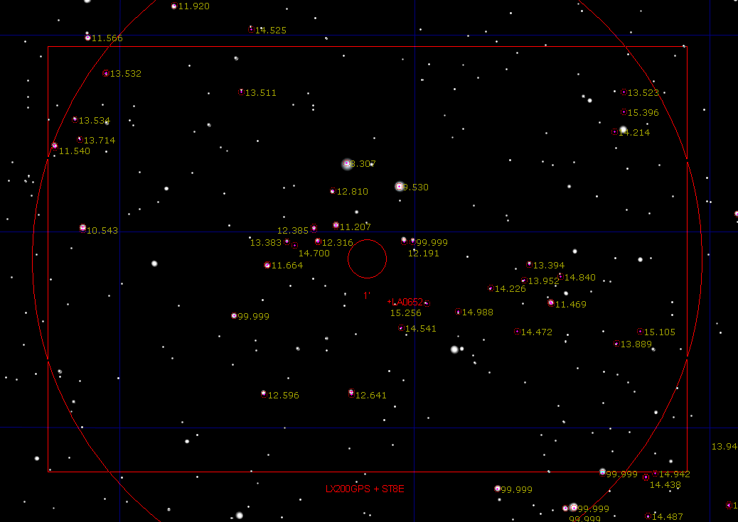
Figure 9. TheSky/Six showing L0652 (Landolt star field at RA
= 06:52) and my telescope system's FOV. Yellow numbers are Landolt R-mag's.
Landolt stars either have BV magnitudes or BVRI magnitudes. By displaying
Landolt R-mag's in TheSky/Six it's easy to see which stars are which; the
BV stars whill show labels of 99.999 whereas the BVRI stars will have real
R-mag labels. This allows for an easy way to position the FOV to maximze the
number of whichever star scategory is desired. If our only goal was to measure
607 V-mag, then the BV stars are as adequate as the BVRI stars. But if we
want to measure 607 BVRI mag's, then we need the BVRI Landolt stars.
For this "Simple First Observation" our goal is to measure 607's V-mag
only. Therefore, all of the stars in the above figure can be used. An observing
plan is to first observe L0652 before 607 reaches elevation 58 degrees (E68
will be my abbreviation for this). Next, we'll observe 607, then back to L0652.
That's all for this observing session.
So far this observing plan consists of 3 sky locations: L0652, 607 and
L0652. Notice that if there are temporal trends in extinction we have reduced
their effect by straddling the target star field with Landolt star field
calibrations. Horizontal gradients is another matter, best left for later.
At each of these 3 sky locations let's take 7 exposures each for filters
V and R. I typically use 10-second exposure times, unguided, which assures
that no Landolt stars are saturated. If the star field has only faint stars
then you'll want to either autoguide and expose longer, or take more than
7 short exposures. Why 7 exposures for each filter? This will be explained
in the next section, but a hint is that it may be necessary to combine sets
of 3 images to improve SNR for the fainter stars, and if one of the 7-image
set is poor quality you can do the 3-image combine twice (and image combine
average these two images for additional SNR).
Summary of this section (Preparing to Observe and Observing Session)
1) Select a night to observe that is "photometric":
cloudless and calm
2) Use a planetarium program (TheSky/Six) to plan the night's observing.
Determine when the target (Region of Interest,
ROI) is at the same elevation as the celestial equator (your "magic elevation")
Determine which Landolt areas are close
to transit at this time.
Choose a Landolt star filed to observe
and note the exact center location that will afford many BV or BVRI stars
within the FOV
3) Perform the night's observations
Near sunset obtain good quality flat fields
(V and R-bands)
Observe the chosen Landolt star field before
it reaches the "magic elevation" (V& R bands)
Observe the target ROI when it's at the
"magic elevation"(V& R bands)
Observe the Landolt
star field again (V& R bands)
MID-LEVEL IMAGE ANALYSIS
The overall image processing scheme is to start with V-band and process
the 7 V-band images of one Landolt star field, then do the same for the other
7 V-band images from the same Landolt star field, then process the 7 V-band
images of the target star field. This will allow us to derive an approximate
V-mag for the target star. That entire procedure is then performed on the
R-band images. This gives us an approximate R-mag for the target star. Finally,
and iteration procedure is performed that solves for the target star's color,
which produces a refined V-mag and R-mag for the target star. This section
and the next (spreadsheet analysis) illustrate the V-band procedure. The same
steps will be used for R-band. The section following the spreadsheet section
describes iteration to solve for target star color.
1) Let's assume that you have 7 images of the L0652 Landolt star field
with V-band. Compare the image with TheSky/Six (I'll assume that's what you're
useing for a planetarium program) and note whcih stars have Landolt magnitudes
(either BV or BVRI). I like to print out an inverted image of the star
field frm a CCD image and hand-note the Landolt magnitudes on it, as shown
in the next figure.
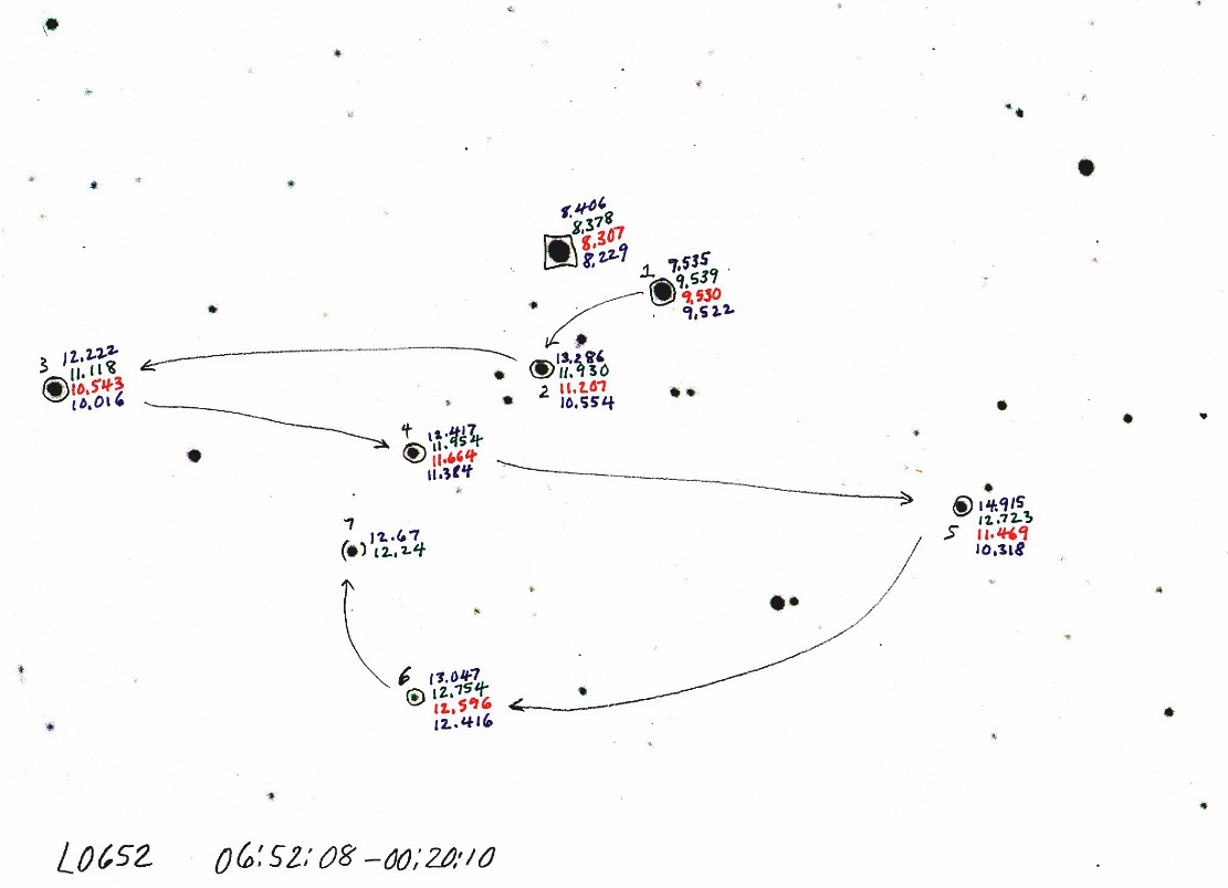
Figure 10. CCD image of L0652 with hand-written Landolt BVRI
magnitudes, as read from the TheSky/Six. The "boxed" star was used as the
"object" in a MaxIm DL photometry reading, and the circled stars were treated
as "check stars." The star numbers and path lines show the sequence for selecting
check stars. The "reference" star is not shown but before photometry readings
were made it was in the upper-left corner. My convention is to start the
path with the brightest and closest BVRI stars and end with BV stars. The
star with a square is the "object" star for MaxIm DL photometry. It serves
the same purpose as so-called "check stars" since they all are available
in the spreadhseet for use in calibrating the telescope system. (The stars
appear fuzzy because this image was made at E22.)
In this figure you'll note that I mapped out a path for doing photometry
readings. This is necessary because when you enter flux readings to a spreadsheet
it will be necessary to know which measured star is associated with which
Landolt star. My practice is to start with the Landolt BVRI stars, and end
with the BV stars. The reason for this will be clear later. In this example
there are 7 "check stars" plus the "object" star. (There's no significance
in these categories since all stars will be used to calibrate the telescope
system.)
2) Review the 7 images using a bright (unsaturated) star for reading FWHM.
Review them again for background sky level (to search for presence of clouds).
If any standout as poor quality, reject them from subsequent analyses. I'll
assume all 7 imagtes are OK for the rest of this tutorial.
3) "Average combine" (using star alignment) the 7 images (this is the
"AV-image"). "Median combine" (using star alignment) the same 7 images (this
is the "MC-image").
An aside: I didn't observe L0652 near transit on this observing session.
Instead, I observed L0558 near transit so I'll use its V-band images as an
example for the rest of this section.
4) Determine a "MC/AV correction" (MC/AV-cor) that places the magnitudes
of the MC-image on the same scale as the AV-image. To do this, read the magnitude
of a star in the AV-image and subtract the magnitude the same star in the
MC-image, record the result somewhere, then repeat this for the other bright
stars. Use the median value of these magnitude differences (if you use the
average difference you might be influenced by a hot pixel or cosmic ray defect
within a signal aperture). Be sure to use a large aperture for this (e.g.,
Ap => 3.5 × FWHM). For example, my L0558 set of 7 V-band images has
MC/AV-cor = +30 mmag.
5) Determine an F-cor plot for the MC-image. To do this read the magnitude
of a bright star in the MC-image using aperture radii 12, 14, 16 ... 30 and
enter these readings in a spreadsheet. Form a column that's the ratio of the
aperture radius to the FWHM of the star being measure (henceforth, I'll use
th term "Ap" in place of "photometry aperture radius"; Ap will have the dimensions
of pixles, abbreviated "px"). Form another column that's the magnitude difference
between magnitude reading at each radius setting and the brightest
magnitude (at the largest Ap setting). This is illustrated in next figure
for L0558, along with a model fit (it's not necessary for you to do the model
fit).
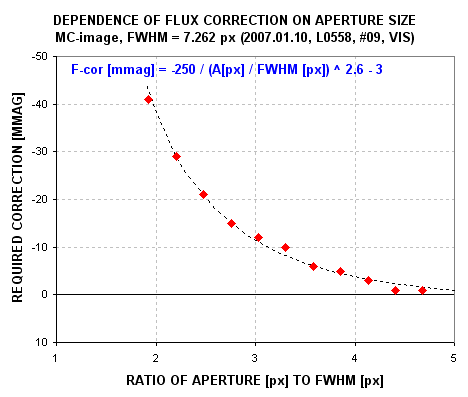
Figure 11. F-cor plot for MC-image (L0558, V-band, #09).
6) Adopt an Ap based on the quality of the F-cor plot. Try to use as small
an Ap as possible to increase SNR, but don't adopt an Ap associated with F-cor
> ~30 mmag because when this level of correction is needed individual stars
withn the FOV may require F-cor values that differ by ~5 mmag. For this example,
when Ap/FWHM = 2.3 the MC-image's F-cor = -25 mmag. Since FWHM for this image
is 7.262 px we may adopt Ap = 17 px. The MC F-cor for this Ap choice is -25
mmag.
7) Hand measure all star fluxes (or see a later section for automatically
measuring them) using the Ap chosen in the previous step. Record the flux
readings in the reduction log.
At this point let's assume that you have in your reduction log a record
of manual flux readings for each Landolt star made from the MC-image for
V-band. In addition, you have a value for "MC/AV-cor" that was determined
by comparing fluxes of bright stars in the MC- and AV-images. Finally, you
have a value for "MC F-cor" based on an Ap choice after inspecting the MC
image's F-cor plot (i.e., the above figure) which must be applied to the
manual flux readings of the MC-image using the chosen Ap.
Summary So Far (Image Processing) ~ 10 minutes (assuming a template
exists froma previous session)
1) Prepare star field finder chart with Landolt
star magnitudes (BVRI) and identifications for "Obj" and "Chk1," "Chk2" etc.
Draw a "path" for the sequence of measurements.
2) Review a set of 7 Landolt images and reject bad ones (big FWHM).
3) Average combine and median combine these images. Call thes AV_image"
and "MC-image."
4) Determine "MC/AV-cor" defined as median difference bewteen magitudes
of bright stars (AV mag - MC mag).
5) Create table of "MC F-cor" versus Ap (aperture rqadius) using the MC-image.
Read mag's for 14, 16, ... 30 px. Record in reduction log.
6) Adopt largest Ap with "MC F-cor" < 20 mmag for next step.
7) Measure fluxes of Landolt stars using the adopted Ap; record in reduction
log.
MID-LEVEL SPREADSHEET
DATA ANALYSIS
The spreadsheet can be organized with a worksheet for V-band and another
worksheet for R-band. It will be useful to have a "scratch" worksheet for
such things as the F-cor data and plot (above figure). The following figure
will be referred to by the next few steps.
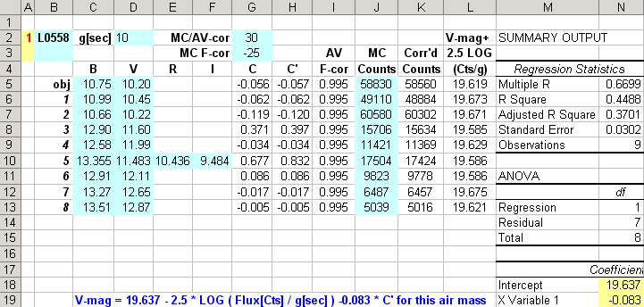
Figure 12. Sample worksheet for manual readings of L0558 V-band
star fluxes. The light blue cells are for user entry. The yellow cells are
significant results.
1) Prepare the V-band worksheet with Landolt magnitudes, as illustrated
by cells B4:F13 in the above figure. Enter values for exposure time, g[sec],
and MC/AV-cor. Star colors in columns G and H should be calculated using the
following algorithms: star color, C:  and C'
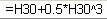
Column I is F-cor calculated from MC-cor using: 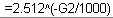
Enter the manual flux readings from the reduction log in column J. The
worksheet should calculate corrected flux by multiplying columns I and J.
Column L is "V-mag + 2.5 × LOG ( Flus [counts] / g [sec] ).
Perform a "least squares regression" using column L as the independent
variable and column H as the dependent variable. The results of this LS regression
are in cells N18 and N19.
Let's review the "magnitude equation" for the case of observing only at
one air mass, which was given in the "Fundamenals and Terminology" section.
V-mag = 19.76 - 2.5×LOG10 ( Stotal
/ g ) - 0.02×C'
(Eqn. 16)
This equation can be generalized in the following manner (using "Flux [counts]"
as equivalent to "Stotal"):
V-mag = ZeroShiftConstant - {2.5 × LOG
(Flux [counts] / 10)} + {StarColorConstant × C'}
(Eqn.17)
where the two parameters in bold are unknown coefficients unique to the
telescope system.
N18 is identified as the ZeroShiftConstant and N19 is identified
as the StarColorConstant.
For this example we have:
V-mag = 19.637 - 2.5 × LOG (Flux [counts] / 10)}- 0.083
× C
(Eqn. 18)
Note that this equation is only valid for the air mass for the set of 7
L0558 V-band images, which was 1.323. If we wanted to generalize this equation
for use with images taken at other air mass values (we won't have to, but
it is interesting to know how to do this) we would have to adopt a value for
zenith extinction. At my site V-band zenith extinction for this season can
be assumed to be close to 0.14 [mag/airmass]. The missing term in the above
equation that would make it useable for all air mass values is - Kv'
× m, where Kv' is V-band zenith extinction and m = airmass.
Since Eqn.12 is for m = 1.323, and since Kv' = 0.14 for my site
at this season, the missing tyerm has the value -0.185. If we apply this to
the zero shift constant and insert the extinction term, we get:
V-mag = 19.822 - {2.5 × LOG (Flux [counts] / 10)}-
0.14 × m - 0.083 × C
(Eqn.19)
This is the equation we would use if we had to use Landolt observations
to calibrate a target star field when the two air mass values were slightly
different. There's no harm in using it when the air mass values are effectively
the same since Eqn. 13 will be equivalent to Eqn. 12 for that case.
If we had observed only this one Landolt star field then we could use Eqn.
12 or 13 to calibrate the target star observations. But since I'm assuming
we have another observation of the same Landolt star field, we should process
it the same way the first one was processed. The two set of coefficients sould
be averaged and for use calibrating the target star field. I'll assume you
will process the other Landolt images now.
................................
OK, you've processed both Landolt star fields and calculated an average
set of coefficients for Eqn. 12 (let's ignore Eqn. 13 since we're assuming
the target is at the same air mass as the Landolt star fields).
For present purposes, assume the averaged solution is:
V-mag = 19.637 - {2.5 × LOG (Flux [counts]
/ 10)} - 0.083 × C
(Eqn.20)
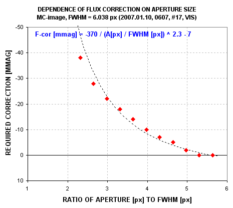
Figure 13. F-cor plot for MC-image (0607, V-band, #17).
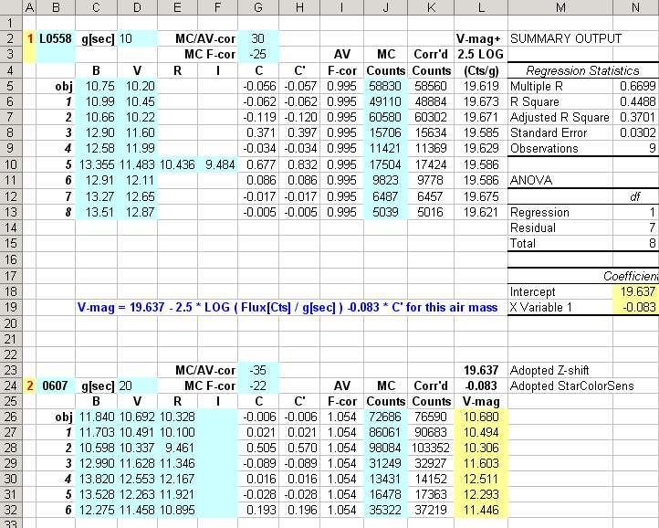
Figure 14. Sample worksheet showing a new section (rows 23 to
32) for representing "0607" measurements.
In this figure the worksheet has default V and R magnitudes in cells D26:E32
from results of a more sophisticated procedure (to be described in another
section below).
Summary So Far (Spreadsheet Analysis) ~ 5 minutes
1) Prepare a spreadsheet with one worksheet per
filter band. Enter Landolt mag's for BVRI in each worksheet.
2) Make sure each worksheet also calculates star colors C and C'
3) Enter values for the exposure times, "MV/AV-cor" and "MC F-cor"
in appropriate cells
4) Be sure that a column exists for a multiplier for the sum of the above
two corrections (column J, in Fig. 4)
5) Enter the hand-measured star fluxes
6) Be sure there's a column that corrects the fluxes for the two corrections
7) Be sure there's a column for V-mag + 2.5 × LOG (Flux / g )
8) Perform a regression analysis using C' as the dependent variable and
the above column as the independent variable
9) Note the solution for the constant and independnet variable coefficient.
These are the "zero shift constant" and "star color constant"
10) Substitute the above two constants in the magnitude equation for same
air mass analyses:
V-mag = ZeroShiftConstant - {2.5 × LOG (Flux [counts] / 10)}
+ {StarColorConstant × C'}
11) After the second set of Landolt star field images have been processed
in an identical manner to the first, average the two sets of constants.
Save this equation for use
with the target star field
12) Prepare a worksheet section below the above Landolt analysis section
that is to be used for the target star field measurements. Since we don't
know star color for the target star (and nearby stars), enter default magnitudes
for V and R that yield C' ~ zero.
13) Process the target data the same way used for the Landolt data, as
far as step 5, above.
14) Be sure there's a column for calculating V-mag (refer to Fig. 6).
This completes the processing of V-band observations.Repeat it for R-band
observations using a separate worksheet.
MID-LEVEL ITERATION
FOR STAR COLOR SOLUTION
By now you should have established magnitude equations for V-mag and R-mag,
and these equatiaons should have been used to calculate the target star's
V-mag and R-mag under the assumption that it has a star color C' = 0.
We now begin an iteration process that will lead to V-mag and R-mag solutions
that rely upon star colors that come from the observational data. Copy the
V-band magnitude solutions tothe R-band worksheet's V-bnad column. Do
the reverse (copy the R-band magnitudes to the V-band worksheet's R-band column.)
The C and C' columns will now be non-zero. The solutions for V-band and R-band
will change somewhat. Repeat the above copying sequence again, and note how
much change has occurred. If the cahnge is less than a mmag then you're done
iterating. If it's larger, repeat the process again, etc.
Voila! You've just performed an all-sky calibration transfer from a Landolt
star field to an unknown target star field!
The next section summarizes results for all bands.
FINAL MAGNITUDES & FINDER CHARTS
_______________________________________________________ x0607
________________________________________________________________
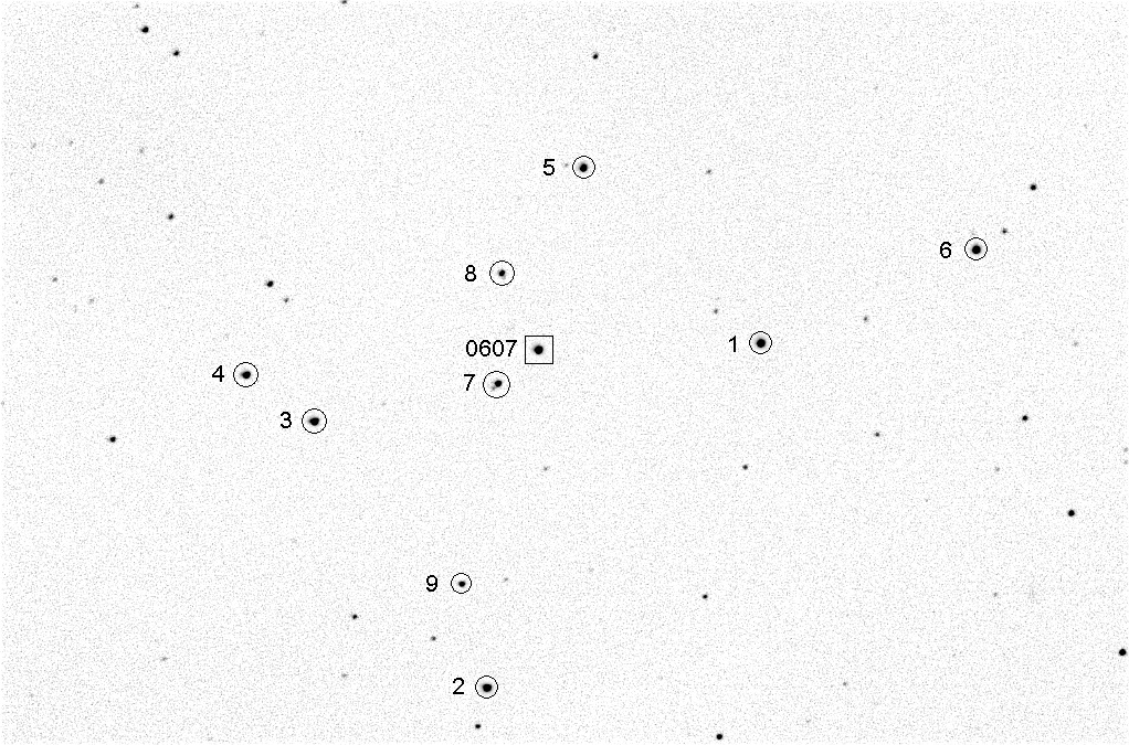
Figure 15. 112p59.0607, FOV = 16 x 11 'arc, north up, east left.
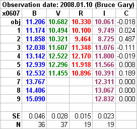
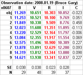
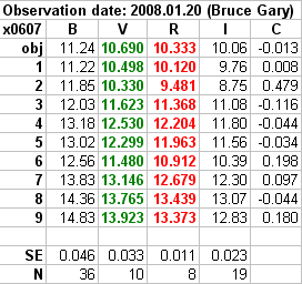
Figure 16. Summary of 3 all-sky observing sessions. Bold colored
entries indicate measurements for that date; unbold B&W entries indicate
concensus of measurements from other dates. The "SE" row is the RMS of Landolt
star measured magnitudes w.r.t. the magnitude equation solution for that filter
and date. "N" is the number of Landolt stars used in the solution.
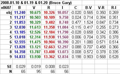
Figure 17. Weighted average magnitudes of x0607 star field using
all-sky measurements from all (3) dates.
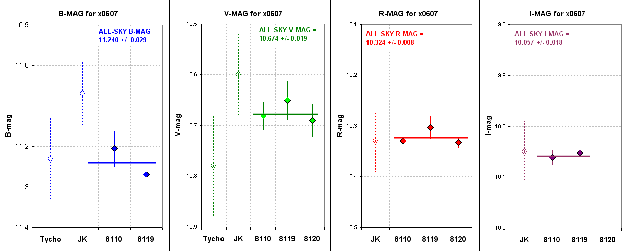
Figure 18. Summary of various magnitude estimates for x0607.
Here's a summary of x0607 all-sky mewasurements.
x0607
B-mag = 11.240
± 0.029 (formal SE)
V-mag = 10.674 ±
0.019 (formal SE)
R-mag = 10.324 ± 0.008
(formal SE)
I-mag = 10.057 ±
0.018 (formal SE)
|
To see a large-format LRGB image of "x0607" for the purpose of verifying
that stars that should be blue and red according to the above table are
in fact blue and red, click LRGB 0607.
_______________________________________________________________ x
2190 _______________________________________________________
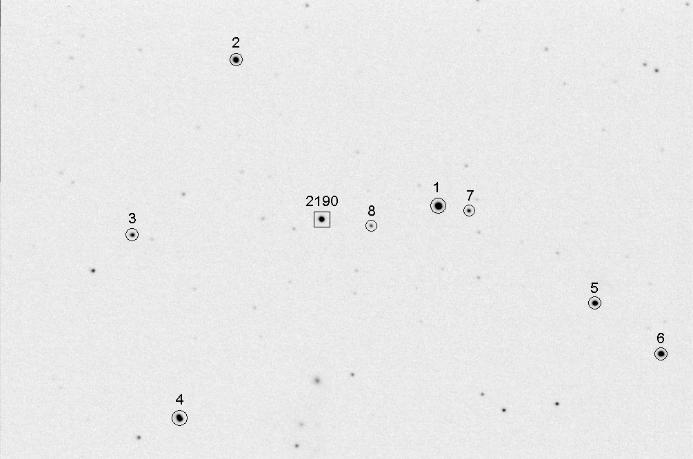
Figure 19. 120p38.2190, FOV = 16 x 11 'arc, north up, east left.
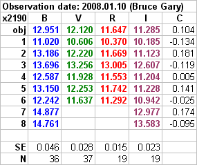
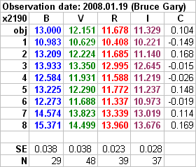
Figure 20. Summary of 2 all-sky observing sessions. Bold
colored entries indicate measurements for that date; unbold B&W entries
indicate concensus of measurements from other dates. The "SE" row is
the RMS of Landolt star measured magnitudes w.r.t. the magnitude equation
solution for that filter and date. "N" is the number of Landolt stars used
in the solution. (The 2008.01.19 imags are currently being processed;
they include BVRI under good sky conditions.)
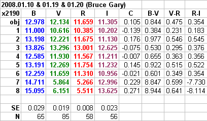
Figure 21. Weighted average magnitudes of x2190 star
field using all-sky measurements from all (3) dates.
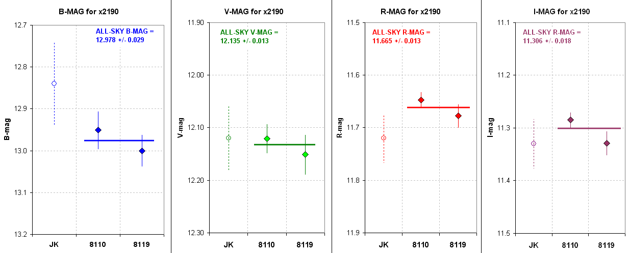
Figure 22. Summary of various V-mag & R-mag estimates
for x2190.
Here's a summary of x2190 all-sky magnitude measurements:
|
x2190
B-mag = 12.978 ± 0.029
(formal SE)
V-mag = 12.135 ± 0.013
(formal SE)
R-mag = 11.665 ±
0.013 (formal SE)
I-mag = 11.306 ±
0.018 (formal SE)
|
To see a large-format LRGB image of "2190" for the purpose of verifying
that stars that should be blue and red according to the above table are in
fact blue and red, click LRGB_2190.
Table I: Number of Landolt Star Fields and Number of Landolt
Stars Used in All-Sky Solutions
Observing Date
|
Landolt
Fields
|
BLU
|
VIS
|
RED
|
INF
|
2008.01.10
|
6
|
36
|
37
|
19
|
19
|
2008.01.19
|
5
|
29
|
48
|
39
|
37
|
2008.01.20
|
2
|
0
|
10
|
8
|
0
|
COLOR-COLOR SCATTER DIAGRAM
There's always one final check when all-sky observations include 3 or more
bands. For example, if BVR are observed we have two ways to describe the star's
color: B-V and V-R. A scatter plot of one color versus the other, overlayed
with a color-color scatter plot for Landolt or Henden stars, can reveal if
a book-keeping error crept into the analysis. With BVRI bands several color-color
scatter plots are possible. Here are some examples for this case study.
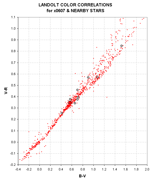
Figure 23. V-R versus B-V for Landolt stars (small red dots),
x0607 (large red square) and nearby stars (gray circles). (Three or four
stars are faint and have poor SNR .)
In this color-color plot it is apparent that the all-sky solutions for
x0607 and nearby stars, as a group, are "compatible" with (main sequence)
Landolt stars. If there are book-keeping errors in the all-sky analysis they
must be less than ~0.02 mag. This plot leaves out I-band; hence the next
plot.
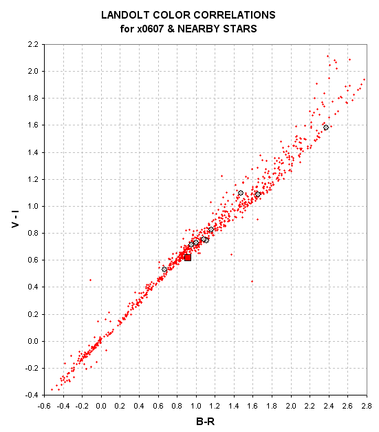
Figure 24. V-I versus B-R for Landolt stars (small red dots),
x0607 (large red square) and nearby stars (gray circles).
Again, when we look at a color-color plot like this the question we should
have in mind is "Do the all-sly measurements as a group fit within
the spread of Landolt points?" The reason "as a group" is important is that
all stars in the unknown star field share the same all-sky calibration for
each band. If the 5 or 6 Landolt star fields used to establish coefficients
for the magnitude equation for a specific band were in error it would cause
all stars in the unknown field to be biased in the same direction, and this
would produce a shift in the above color-color plot away from the centroid
of Landolt star colors. In this case, for V-I versus B-R, the group of unknown
stars agree with the Landolt stars. Since this color-color plot involves
all four filter bands it constitutes a persuasive argument that all filter
bands were correctly calibrated. The fact that one of these stars, x0607,
appears to be slightly "off" the Landolt meadian of points simply means that
this star has colors slightly different from the Landolt stars inthis color
region.
Here are the corresponding plots for x2190.

Figure 25. V-R versus B-V for Landolt stars (small red dots),
x2190 (large red square) and nearby stars (gray circles).
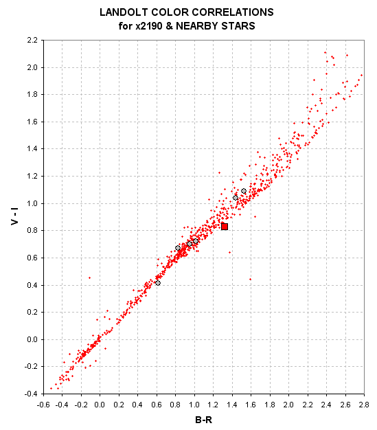
Figure 26. V-I versus B-R for Landolt stars (small red dots),
x2190 (large red square) and nearby stars (gray circles).
UPPER-LEVEL IMAGE ANALYSIS
The previous results were in fact based on an all-sky analysis procedure
that is a little more involved than the one described in the "MID-LEVEL ANALYSIS
section. This section describes what I actually did; it should only be read
after the previous sections have been read and understood.
UPPER-LEVEL SPREADSHEET
ANALYSIS
Deriving V and Rc
from r' and JK
If you have a r'-band filter (an Rc filter will probably work also), here's
an option that should interest you. Stars with r'-band calibration are all
over the sky, and asteroid people use them all the time. The calibrated r'-band
stars are in the Carlsberg Meridian 14 Catalog. For my asteroid work
I've never failed to find lots of Carlsberg r'-band stars in every FOV, which
is important for long period asteroids that move from one FOV to another every
night. It's easy to see which stars in a FOV are in the Carlsberg catalog
using the free program DS9 (explained below). Almost all stars also have 2MASS
J and K magnitudes. The relationship between V and r' is pretty well established
if you have the J-K color. The relation between Rc and r' is even more accurately
established with the J-K color. The relation between Ic and r' exists, but
it's not good enough; using only J and K gives a better result. Here are
the two relationships (using the first half of stars that are completely
calibrated atthe following bands: u'g'r'i'z' and BVRcIc and JHK).
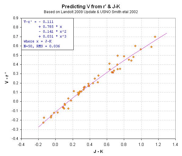
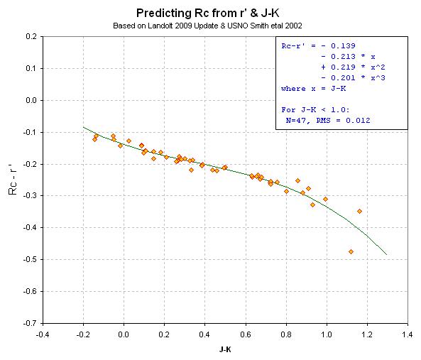
Figure 27a and b. Color/color diagrams for deriving V and Rc from
r' and J-K color.
These two color/color scatter plots show that if you have r' for a star
then you can calculate V and Rc for that star once you get J and K from somewhere.
TheSky/Six has J and K magnitudes for almost all stars; just click on the
star and select the pull down menu for UCAC2. Unfortunately, TheSky/X doesn't
display J and K this easily (it must be possible but I haven't figured it
out yet).
The hard part is getting r' for the target star. I'll show how using an
example. Consider a mystery star field that was observed with 3 exposures
using a r'-band filter. Using MaxIm DL I calibrated each image (dark and
flat), star-aligned them, and produced a median-combined master image. I
used PinPoint to astrometrically calibrate the master image. I then ran DS9
(a free downloadable program: http://hea-www.harvard.edu/RD/ds9/
), navigated my computer's directory structure to the location of the master
image, loaded the image (set Scale to "Z scale") opened the "Analysis" menu,
selected "Catalogs", selected "Optical", selected "Carlsberg Meridian 14".
About a second later all stars in the FOV that were in the catalog were circled,
and a list of magnitudes was displayed in another window (shown in next two
figures).
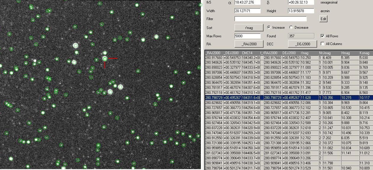
Figure 28a and b. FOV is 10 x 10 'arc (north up, east left for
this mystery field). DS9 cicles stars with Carlsberg Meridian 14 Catalog r'-band
magnitudes. The list on right is highlighting a star with r'-mag = 11.628;
J and K magnitudes are included in the listing. When this row is highlighted
a blinking circle in the image on left indicates which star is highlighted.
I added the two red lines showing the highlighted star, which also is the
"target" star.
The user may decide to accept the Carlsberg Meridian 14 Catalog magnitude
for the target star (assuming it's included in the list). For the case under
consideration the target star has r'-mag = 11.628, J = 10.356 and K = 10.117
(so J-K = 0.239). Using the equations for converting r' and J-K to V (shown
in Fig. 27a) we arrive at V = 11.697 ± 0.047 (the SE was calculated
to be the orthogonal sum of 0.023 and 0.036 and 0.020, corresponding to an
estimate of the Carlberg catalog SE, the SE from the equation in Fig. 27a,
and the SE from uncertainties in J and K). An equation for deriving Rc from
r' and J-K is given in Fig.27b. For this target we calculate Rc = 11.448
± 0.026 (where SE is orthogonal sum of 0.023, 0.012 and 0.005.
If the target's r' is not listed (for some rare reason), or if you want
to use an improved value for the target's r', you can perform a photometry
analysis of the r'-band images of this star field. Since DS9 shows r'-mags
for stars in the FOV you may use them as reference stars when doing the photometry
measurement of the target. It's convenient to print an inverted image of
the star field and label stars with their r'-mags. When I did this for a
3-image set I get r' = 11.645 ± 0.009 (SE is 0.023 / sqrt(N-1)),
and using the conversion equation in Fig.27a yields V = 11.714 ± 0.042
(SE is orthogonal sum of 0.009, 0.036 and 0.020).
A similar procedure yields Rc = 11.465 ± 0.017.
How did we do? This star field is one of the standard star fields with all
bands carefull measured by professionals. Therefore we can compare the above
derived V and Rc magnitudes with true magnitudes. Here are the comparisons:
V from r'JK
= 11.714 ± 0.042
V from Landolt (2009) = 11.733 ± 0.002 (estimated
SE)
V error
= -0.019 ± 0.042
Rc from r'JK
= 11.465 ± 0.017
Rc from Landolt (2009) = 11.400 ± 0.002
(estimated SE)
Rc error
= -0.065 ± 0.017
The V-mag looks good, but the Rc mag is too faint by ~ 4-sigma. use
this procedure at your own risk!
APPENDIX A: PSF SHAPE EFFECTS (FLUX RECOVERY
FRACTION ANALYSIS)
[This section is incomplete, so I recommend not reading
it now]
For amateurs, one of the most difficult aspects of measuring star fluxes
accurately is related to the fact that a photometry aperture never records
the total flux associated with a star. Even if a star had a perfectly Gaussian
point-spread-function (PSF) a circular aperture with a finite radius would
not capture all the flux since a Gaussian function never reaches zero as distance
from center increases. A real-world PSF will usually have broader "skirts"
(far out, low response levels) than a perfect Gaussian; which is to say that
at any given distance far from the star center the brightness will be greater
than a Gaussian fit. For amateurs the PSF is often affected by imperfect
tracking as well as poor seeing. Tracking imperfections usually broaden the
PSF in the RA direction more than the Declination direction. Seeing can cause
the PSF to spread by different amounts at different locations in the FOV,
especially if the exposure time is short. If focus is incorrect, or collimation
is imperfect, the PSF shape will vary across the FOV, being worse near the
edges, usually.
All of these problems are more likely to affect amateurs than professionals,
because amateur hardware is less perfect, seeing is worse and the software
for measuring fluxes is simpler. The software issue is the most important
to understand because it represents a challenge that an amateur might address.
We can't do anything about atmospheric seeing at our low altitude sites, and
we can't do much about imperfect tracking, but we can do something about how
we measure star flux.
The optimum way to process an image to extract a star's flux is to perform
PSF-fitting on all stars in an image and mathematically integrate the PSF
function to arrive at a "volume" for each star. The "volume" should be proportional
to the number of photoelectrons released by the star. This assumes that the
PSF is approximately Gaussian, and if the PSF function allows for azimuthal
assymetry then even if RA tracking was poor, or seeing produced a non-circular
PSF, these effects would be "fitted" in a way that is adequate (to first
order), or at least better than using a simple circlar photometry aperture.
The professionals use PSF-fitting for everything, and in theory some of their
software is available to amateurs. But it's not easy to learn and it doesn't
run on operating systems used by most amateurs, so the remainder of this
appendix will be devoted to uses of aperture photometry that cleverly overcome
its worst shortcomings.
I'll demonstrate some of the problems with using photometry apertures with
real-world amateur PSFs using an image made with my 14-inch Meade LX200GPS
on 2008.01.10. The next image was made using a V-band filter with a 10-second
unguided exposure of the L0558 Landolt star field. The air mass is 1.32.
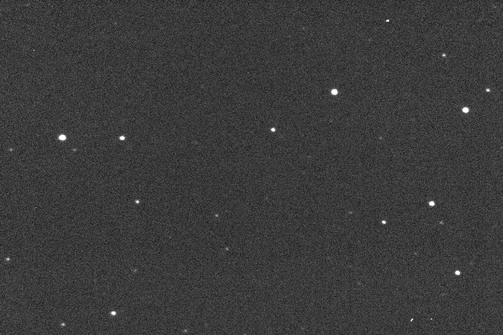
Figure A01. Landolt star field L0558 using V-band filter for
an unguided 10-second exposure. FOV = 16 x 11 'arc. Focus is good but seeing
is average, producing PSF with FWHM = 3.0 "arc for all stars. (Good seeing
produces images with FWHM ~2.1 "arc, so the 3.0 "arc FWHM of this image means
that the PSF is seeing dominated.)
In this image notice that the "bright" stars appear to be "larger." This
effect is produced by the fact that for bright stars the PSF skirts are brighter
than the CCD's noise level. In other words, since we can assume that the fainter
stars have the same PSF they produce photoelectrons beyond the apparent edges
of what our eye perceives. We are familiar with a very bright star
that saturates a CCD image appearing much larger than a bright but unsaturated
star. Try to get used to the fact that every star's PSF extends "forever"
and we're only seeing the "tip of the iceburg."
This appendix consists of a series of "explorations" of the PSF skirt problem
as it affects photometry aperture measurements. The first question I want
to address is: Do all stars in an image have the same PSF? If they do, then
aperture photometry measurements for all stars should suffer the same flux
recovery loss. I will use the above image and perform aperture phtometry measurements
of the 4 brightest stars using a set of aperture circle radii. If all stars
have the same PSF shape then they should require the same "F-cor" (defined
as the magnitude correction required to convert a magnitude measurement with
a small aperture to the magnitude it would have using a large aperture).
The F-cor adjustments are always negative (producing a slightly brightened
star), but I will plot them as positive numbers. Note that the 4 brightest
stars are located at many parts of the FOV: the upper-middle, the upper-right
edge, the left edge, and the lower-right edge. Whatever behavior we learn
about F-cor from this image can be used to characterize exposures as long
as 10 seconds, using a properly focused telescope under seeing conditions
where PSF is dominated by seeing variations during the exposure (instead of
optical imperfections).
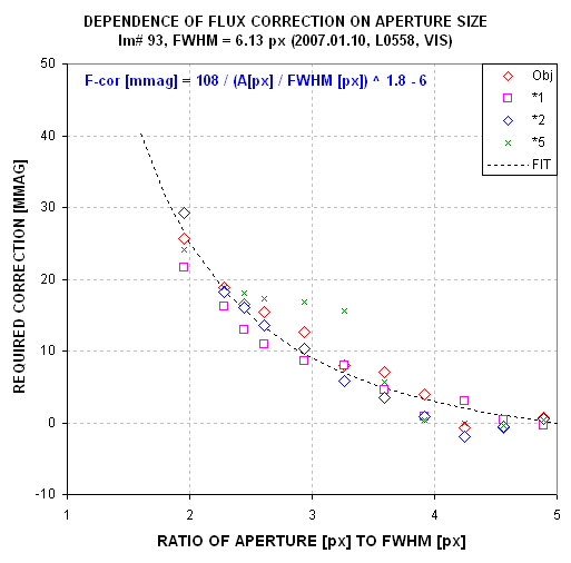
Figure A02. F-cor plot for 4 stars in image #93 which has FWHM
= 6.13 px. The sameness of all stars in different parts of the FOV indicate
that an image can be represented by just one F-cor function. (Star #5 is faint,
with SNR<50, which accounts for its higher noise level.)
This graph shows that all stars in the image have the same PSF. This is
useful information.
If we require that F-cor be less than 5 mmag, this image should be processed
using an aperture of 22 px (3.6 ×6.13).
What about an image of the same star field taken a few seconds later when
seeing and tracking errors were different? Since we've just shown that F-cor
is the same for all stars in the same image (when focus is good and exposure
time is as long as 10 sec), it's not necessary to measure more than one star
in any image to assess it's F-cor requirement. I'll process the bright star
"Obj" (middle-upper-right in FOV).
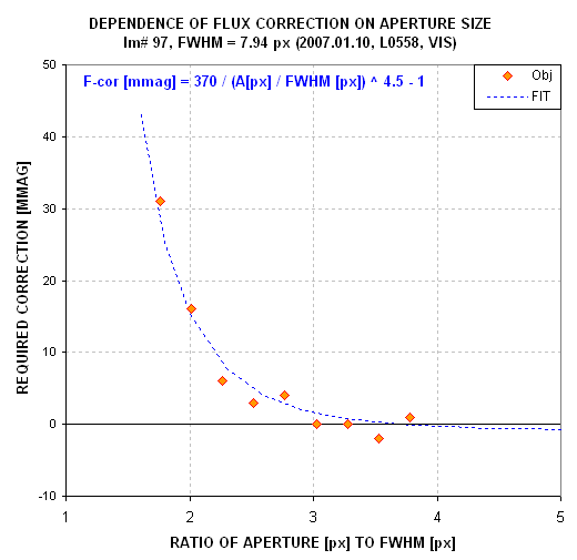
Figure A03. F-cor plot for star "Obj" in image #97 which has
FWHM = 7.94 px.
This F-cor shape is different from the previous one, taken a few seconds
earlier. The shape is different from the previous image's F-cor shape. Apparently
the PSF skirts are varying in ways that are not apparent by looking at the
images or noting their FWHM. If we require that F-cor be less than 5 mmag,
this image should be processed using an aperture of 17 px (2.2 ×7.94).
Isn't it curious that this image, which is less sharp, can be measured with
a smaller aperture than the previous image while satisfying the requirement
that F-cor < 5 mmag. From this we must conclude, reluctantly, that image
sharpness matters when using an F-cor equation to correct measured star fluxes
for finite photometry aperture size.
What's an amateru to do who doen't have PSF-fitting software? It's not
feasible to construct F-cor plots for every image of a night's observing
session! One possibility is to combine a set of 7 images (for a Landolt star
field and filter), and then construct a F-cor plot for that image. This F-cor
plot can be used to adjust star flux readings of the combined image. There
are two principlal ways to combine: median and average. Let's assess the
merits of both.
Let's evaluate the merits of doing the following:
1) Quickly review the 7 images for FWHM of a bright star. Quickly review
them again for background sky level (to search for presence of clouds).
2) "Average combine" (using star alignment) the 7 images (this is the "AV-image").
"Median combine" the 7 images (this is the "MC-image").
3) Determine a "MC correction" (MC-cor) that places the magnitudes of the
MC-image on the same scale as the AV-image. Read the magnitude of a star in
the AV-image and subtract the magnitude the same star in the MC-image, record
the result somewhere, then repeat this for the other bright stars. Use the
median value of these magnitude difference. Be sure to use a large aperture
for this (e.g., Ap => 3.5 × FWHM). For example, the above image
has MC-cor = +30 mmag.
4) Determine an F-cor plot for the MC-image (see Fig. A04).
5) Adopt an aperture radius based on the quality of the F-cor plot. Try
to use as small an aperture as possible to increase SNR, but don't an aperture
with F-cor > ~30 mmag because individual stars withn the FOV may require
F-cor values that differ by ~5 mmag at this level of correction (just a guess).
For this example, F-cor = 30 mmag when Ap/FWHM = 2.2, and since FWHM for this
image is 7.926 px we may adopt Ap = 17 px. The F-cor for this aperture radius
choice is 27 mmag.
6) Hand measure all star fluxes (or see a later section for automatically
measuring them), and record on the reduction log.
7) Enter these fluxes in a spreadsheet devoted to this all-sky observing
session.
8) Convert the fluxes to magnitude (see a later section). Add the F-cor
determined above to these magnitudes. These are the magnitudes that will
be used in solving for telescope system magnitude equations for this filter
band.
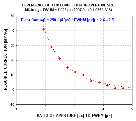
Figure A04. F-cor plot for MC-image.
As an aside, it should be obvious that an F-cor plot from one night cannot
be used for other nights since they vary from image to image in a quick succession
of short exposure images. The following F-cor plot illustrates the difference
between a windy day (upper data & trace) and a calm day lower data &
trace).
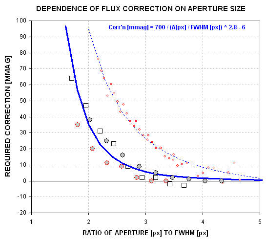
Figure 3a. Flux recovery correction (F-cor) versus ratio "photometry
aperture / FWHM." The upper set of data & its fit are from one date
(windy) and the lower one is from another date (calm), with difference PSF
shapes. The equation in the graph is for the upper data set. The lower data
set is fit by the equation Correction [mmag] = 800 / (ratio^4.5).
In order to construct such a graph we must use a star with high SNR, such
as 1000, in order to assure that we can measure the effect of the star's PSF
"skirts" as we increase the signal aperture. I suggest that you median combine
using star alignment the set of 7 images for a Landolt or target field. Choose
a bright, unsaturated star to work with. Measure the star's FWHM. Set your
signal aperture to ~1.6 times FWHM. For example, if the star has FWHM = 3
pixels, start with an aperture radius of 5 pixels. Set the gap so that its
width is at least this wide (For MaxIm DL you set the ggap width directly,
for AIP4WIN you specify the gap's outer radius.) Set the sky background width
to also be at least this wide. Center the photometry circles on the star
and read the magnitude displayed in the information window. Record this magnitude
along with the signal aperture width (for later entry to a spreadsheet). Increase
the signal aperture radius (leaving the gap and sky background setting alone),
and record the aperture and magnitude again. Only magnitude changes are important
for this exercise, so don't worry if the magnitudes are wildly offset from
what they should be. Note that when the aperture radius is increased the
magnitude decreases (i.e., the flux within the signal aperture increases).
Keep track of this change each time you increase the aperture. Repeat the
aperture increases and recordings until the magnitude no longer decreases.
We'll call this the asymptotic magnitude, and it will be close to the total
flux that can be recovered from this star image. You can expect that the
largest aperture needed for total flux recovery will be about 5 times FWHM.
If you want, you may increase the aperture in 2 pixel increments.
Enter the set of readins of magnitude and signal aperture radius in a
spreadsheet. Add a column for the difference between magnitude reading and
asymtote magnitude. Add another column for ratio of aperture to FWHM for
the star. Plot these two columsn in a graph like the one above. If you want,
overplot a model that fits the data; it can have the form f-cor = Constant1
/ (ApertureRadius / FWHM ) constant2. I'll refer to such a graph
as an "f-cor plot for a 7-image set." This plot can be used to guide us in
how small an aperture can be used without risk of introducing more errors
than we want as we try to increase SNR for the faint Landolt stars by using
small apertures. Note that our goal is to achieve a telescope system calibration
accurate to 0.020 magnitude, or 20 mmag. If we use an aperture that calls
for an f-cor of 20 mmag, for example, it is unlikely that we will be introducing
errors as large as 20 mmag. Based on the deviation of the plotted data in
this graph with the model fit it is likely that a 20 mmag correction will
have errors of 5 or 10 mmag. This amount of error is acceptable. As several
stars are to be corrected using the model fit some will have "+" errors and
others will have "-" errors, and the average error will be even less.
Using the above "f-cor plot for a 7-image set" in the above figure the
solid blue trace model fit guides us to the use of a signal aperture ~2.2
to 2.5 × FWHM. If FWHM = 3 pixels, then we are allowed to use aperture
as small as 7 pixels for measureing fluxes from this 7-image set.
4) For this first image analysis exercise I'll ask you to hand-measure
star fluxes. Later, after you understand the concepts related to what's done
with these fluxes, you can automate the flux measurements with phtometry
tools in MaxIm DL and AIP4WIN. (In a later lesson I'll also suggest that
if you're using MaxIm DL add an "artificial star" in the upper-left corner
of each image. This is very useful, and time-saving, because it can be used
as a "reference star" with the same flux for all-time: 1,334,130 ADU, for
the 64x64 version.)
This paragraph is an aside. It's possible to hand-measure all Landolt
star fluxes for later entry into a spreadsheet, and for a couple years I
did it this way. The main purpose in using the photometry tool to automatically
measure fluxes and create a CSV-file is to save time. A second reason for
doing it is to produce higher quality fluxes by virtue of the fact that the
photometry tool rejects bad pixel readings form the sky background annulus
whereas the hand readings don't (MaxIm DL is working on this for a future
version). Our objective in this image analysis section is to create a set
of readings that can be read into a spreadsheet for convertion to fluxes.
It is permissible for this "Simple First Image Analysis" to record hand readings
of star flux for each Landolt star in each image for later hand-entry into
a spreadhseet.
So, this step consists of hand-measuring the flux of each Landolt star
using the aperture chosen in the previous step (e.g., 7 pixels, or whatever
it was). Careful book-keeping is important since the hand-recorded fluxes
will be entered into a spreadsheet. Record the FWHM for a bright star for
each of the 7 images. In the spreadsheet we will assume that all stars in
an image have the same FWHM. This won't be true, but it's a good first approximation.
The FWHM associated with each image can be used to calculate an f-cor to be
applied to all fluxes from that image.
Maybe you're wondering why it's necessary to record FWHM for each image.
It's only necessary if you use a signal aperture radius that's smaller than
4 × FWHM. For example, my FWHM is typically 5 pixels, and if I wanted
to neglect the "flux recovery correction" I would have to use an aperture
radius of at least 20 pixels. There are penalties for using such a large aperture.
SNR is lower the larger the aperture, and when only faint Landolt stars are
present this can be an important penalty. Another penalty occurs when another
star is nearby and could be included in the aperture when it is this large.
Every situation is unique so this is something that each all-sky observer
will have to experiment with. In fact, the more I write about this the more
I think you should at least once do a manual flux reduction.
____________________________________________________________________
WebMaster: Bruce
L. Gary. Nothing
on this web page is copyrighted. This site opened:
2008.01.10 Last Update: 2010.09.16