Abstract

This web page describes a method for achieving all-sky photometry with an accuracy of ~0.04 magnitude. It employs a procedure that is much simpler to understand and implement than the standard one. Some theoretical background is included so that the reasons for procedures can be understood. For observers content with phtometric accuracy no better than ~0.10 magnitude I recommend a different web page (http://brucegary.net/dummies/x.htm) since the all-sky iterative procedure requires a lot of work with manual measurements and spreadseheet analysis.

    Fundamentals
    Observing Strategy Considerations
    Iterative All-Sky Analysis Procedure - Initial System Calibration
    Subsequent All-Sky Photometry
   Differential Photometry Iterative Procedure (DPIP)
    DPIP for Dummies (for the impatient observer who wants to try out DPIP right away)    

INTRODUCTION

If the earth didn't have an atmosphere that absorbs starlight then all-sky photometry would be trivial. The observer would merely take a CCD image of a region with well-calibrated stars, then another image of the region of interest with the same settings. Corrections would still be required for the observing system's unique spectral response, but these "transformation corrections" would be straightforward since they wouldn't depend on air mass or weather conditions.

Some observers frequently encounter the need for an accurate magnitude scale in a region devoid of well-calibrated stars. For example, asteroids are constantly moving through parts of the sky that do not have nearby well-calibrated stars. Anyone wanting to determine the BVRI spectrum of an asteroid is "on his own" for establishing accurate magnitudes for stars near the asteroid. Novae and supernovae are the most common examples of stars that appear where there are no well-ccalibrated stars. When a bright one of them is discovered the AAVSO does a good job of quickly preparing a chart with a magnitude "sequence" that is based on observations quickly-arranged for by a professional astronomer (Arne Henden) who uses "all-sky photometry" to establish the sequence. Not every nova or supernova can be supported this way.

Because of the growing number of amateurs with CCD skills conducting projects that involve accurate brightness measurements there is a growing need to explain how to perform all-sky photometry. I have encountered enough situations where I needed to create my own "photometric sequence" chart that I have been motivated to learn all-sky photometry techniques. In the process of this learning I have developed what I believe is a straight-forward method for all-sky photometry. Maybe it is the same as used by the professionals, but I'll admit to not having determined this yet.

When I started writing this web page I thought I would try to discourage amateurs from trying to do all sky photometry. I had many concerns about the feasibility of an amateur astronomer taking on a task that required sophisticated observing strategies and data analysis. (This may sound funny, coming from an amateur, but I spent decades as a radio astronomer and atmospheric scientist, where I became familiar with atmosperhic extinction and data analysis methods.) I was especially concerned about the amateur being blindly misled in his analysis by spatial inhomogeneities and temporal variations of atmospheric properties (which I had studied before my retirement). I was prepared to advise amateurs to restrict themselves to "differential photometry," which is based on a single image of the region of interest. However, while I was learning to do all-sky photometry for my own projects I developed a procedure which I now believe makes it feasible for other amateurs to make their own chart sequences using a version of "all-sky photometry" that I am calling "Iterative All Sky Photometry." My purpose for this web page has thus changed from trying to discourage amateur astronomers from doing all-sky photometry to trying it using a technique that I think is within the reach of many amateurs.

The observer who is impatient may click the link "Observing Strategy" or "Analysis Procedure" given above. For those wanting some grounding in fundamentals, however, I begin with a section that reviews atmosphere absorption, as well as difficulties related to temporal variations and spatial inhomogenieties of atmospheric properties.

Finally, if your goal is to achieve photometric accuracies no better than ~0.1 mag, I recommend a web page that I prepared for amateurs whose main interest is asteroid astrometry but who wish to improve over the 1 or 2 magnitude errors that are commonly prepared by automatic programs (such as PinPoint) for submission to the Minor Planet Center. This web page can be found at Photometry for Dummies. This web page is meant for those wanting to achieve 0.04 magnitude accuracy.

FUNDAMENTALS

Flux

First, imagine that you're out in space, holding a magic "unit surface area" so that it intercepts photons coming from a star. The surface can be a 1 meter square, for example, and its magic property is that it can count photons coming through it for any specified interval of wavelengths, for any specified time interval. Let's give it one more magical property:  it can count only those photons coming from a specific star that you designate.  We might imagine that this last is achieved by some kind of screen way out in front, having at least the same 1 meter square aperture and located so that the magic surface sees only things from the direction of the star.

This device measures something commonly thought of as brightness, but which astronomers call "flux." Photons of the same wavelength have the same energy, so merely counting photons is equivalent to measureing the energy passing through the magic unit surface. Energy per unit time is power, as in "watts."  This magic device measures watts of energy, per unit area, per nanometer of wavelength interval. This is called flux, or a version of flux referred to as S_lambda. Let's just call it "S".

Magnitude

If we point our magic unit surface area so that we measure S from one star, then S from another, we'll get two S values:  S₁ and S₂. We can arbitrarily define something called "magnitude difference" according to the following:  M₂ - M₁ = 2.5 * LOG₁₀ (S₁ / S₂ ).

Let's now arbitrarily assign one star to have a magnirude value of zero. Then, all stars brighter will have negative magnitudes, and all stars dimmer will have positive magnitudes. If the flux from that universal reference star is S₀ , then any other star's magnitude will be given by:  

    M_i =  2.5 * LOG₁₀ (S₀ / S_i )                Eqn 1

We've now devised a system for describing how many photons pass through a unit surface area, per unit time, per wavelength interval, at a specified interval of wavelengths. And we've arbitrarily devised a dimensionless parameter, called "magnitude," for the convenient statement of that number. Magnitude defined this way is convenient because we don't have to give a long value, such as 1.37e+16 [photons per second, per square meter, between 400 and 500 nanometers]; rather, we can simply say M = 12.62.

But wait, we're not done. The wavelength interval is a crucial part of the measurement, since the measurement will vary greatly as we change wavelength intervals. Let's just call the meaurement for the 400 to 500  nanometer (nm) wavelength region a "blue" magnitude. And we can define "green" magnitudes, and "red" magnitudes, etc, by specifying the wavelength region to be 500 to 600 nm, 600 to 700 nm, etc.

Atmospheric Transmission

Now let's take our magical instrument from outer space down through the atmosphere to the surface of the earth. When we look up, we will count fewer photons. Some of the photons are being absorbed by molecules in the atmosphere, and others are being scattered. The scattering is from two kinds of things:  molecules and particles. The molecules scatter in a Rayleigh manner, affecting blue photons most, whereas the particles (also called aerosols) scatter in a way that depends upon the ratio of the wavelength to the circumference of the particle (Mie scattering when this ratio is small, Rayleigh scattering when the ratio is large). At some wavelengths, especially within the "red" band, water vapor molecules absorb (resonant absorption) at specific wavelengths. Ozone molecules also have a preferred wavelength for absorbing photons. For these bands the loss of photons will depend upon the number of water vapor molecules, or ozone molecules, along the line of sight through the atmosphere.

To first order, the loss of photons making a straight line path to the magic unit surface area, located at the surface of the earth, will depend on the following factors:

    Blue        Rayleigh scattering by molecules, non-resonant absorption by molecules, scattering by aerosols
    Green      Non-resonant absorption by molecules, scattering by aerosols
    Red         Non-resonant absorption by molecules, scattering by aerosols, water vapor molecules resonant absorption

Let's talk more about the aerosols. They may consist of dust particles, salt crystals that are swollen by varying amounts of absorbed water (these are important at coastal sites), sulphate particles (SO₄ molecules stuck together plus with water), volcanic ash in the stratosphere, urban smog, water droplets within clouds, and ice crystals in cirrus clouds. All of these aerosols are capable of presenting angular structure that can pass through a line of sight quickly, such as between the measurement of one star and the next. Even during clear conditions, when the eye cannot see changes in water vapor, the total number of water vapor molecules along a given line of sight can change by a factor of two in less than an hour (personal observation).

The zenith view will usually have the smallest losses. During a typical observing period the entire sky will undergo a uniform rate of change of all of the above factors contributing to loss of photons. Tracking an object from near zenith to a low elevation will cause photon losses to change due to both the increasing amount of air that the photons have to traverse, and due to the changing conditions of the entire air mass in the observer's vicinity. We'll have to come back to this pesky subject later.

If the atmosphere in the observer's vicinity does not change during an observing sesson, then the photon losses will be proportional to the number of molecules and aerosols along the path traversed by the starlight. The losses are exponential, however. Each layer of the atmosphere absorbs or scatters a certain percent of the photons incident at the top of that layer. For example, if the zenith flux is 90% of what it is above the atmopsphere, the 30 degree elevation angle flux (where twice as many air molecules and aerosols will be encountered) will be 90% of 90%, or 81% of the outer space flux. Simple geometery says that:

    S(m) = S(m=0) * EXP{-m * tau)                Eqn 2

where S(m) is the flux measured for an air mass value "m", S(m=0) is the flux above the atmosphere, "EXP" means take the exponential of what's in the parentheses, and "tau" is the optical depth for a zenith path. Tau, the zenith extinction, can is sometimes assigned units of "Nepers per air mass." (Apologies to astronomers accustomed to seeing air mass represented by the symbol "x"; I'm going touse "m".)

The following figure shows atmospheric transparency for a clear atmosphere with a moderatley low water vapor burden (2 cm, for example).

Figure 1.   Atmospheric transmission versus wavelength for typical conditions (water vapor burden of 2 cm, few aerosols), for three elevation angles (based on measurements with interference filters by the author in 1990, at JPL, Pasadena, CA). Three absorption features are evident:  a narrow feature at 763 nm, caused by oxygen molecules, and regions at 930 and 1135 nm caused by water vapor molecules. Four thick black horizontal lines show zenith transparency based on measurements made (by the author) with a CCD/filter wheel/telescope for typical clear sky conditions on another date and at another location (2002.04.29, Santa Barbara,CA, SBIG ST-8E, Schuler filters B, V, R and I).

Since zenith extinction changes with atmospheric conditions differences of several percent can be expected on different days. In Fig. 1 the transparency in the blue filter region (380 to 480 nm) differs by ~10% between the two measurement sets. Changes of this order can occur during the course of a night. This may be an unwelcome thought, but it is a fact that careful photometry must reckon with (discussed below).

At my new observing site in Southern Arizona (4660 feet elevation) I have measured the following extinction constants (2004.10.15):

        B = 0.28 magnitude/air mass, or 77 % zenith transmission                 
    V = 0.16              "                or 86 %           "
    R = 0.13              "                or 89 %           "
    I = 0.09              "                or 92 %
    C = 0.13              "                or 89 %           "     (i.e., unfiltered)

Unsurprisingly, a medium-high altitude site in Southern Arizona has less extinction thatn a coastal site in Southern California.

Hardware Spectral Response

The concept of "spectral response" is important throughout all that is dealt with here, so let's deal with that now. Consider a single observation (or integration) of a field of interest using a single filter. The term"spectral response" refers to the probability that photons of light having different energies (wavelengths) will successfully pass through the atmosphere (without being scattered or absorbed) and pass through the telescope and filter and then be registered by the CCD at some pixel location. This probability versus wavelength, called spectral response, varies with photon wavelength, ranging from zero at all short wavelengths, to maybe 20% (as described below) near the center of the filter's response function, and back to zero for all longer wavelengths. The spectral response will be a smooth function, having steep slopes on both the short-wavelength cut-on and long wavelength cut-off sides of the response function. The entire journey of a photon through the atmosphere, the telescope, the filter, and it's interaction with the CCD chip, where it hopefully will dislodge an electron that will later be collected by the CCD electronics when the integration has finished, can be summarized by "probability versus wavelength" functions, described next.

Assuming the observer is using a reflector telescope, or a Schmidt-Cassegrain with small losses in the front glass corrector, the photon that makes it to ground level has a lossless path through the telescope to the filter. For observers using a refractor telescope, there may be losses in the objective lens due to reflections and absorptions. For a good objective, though, these losses will be small.  The remainder of this section deals with what happens to ground-level photons that reach the filter.

Filter Pass Bands

There are two commonly used UBVRI filter response "standards" in use, going by the names Cousins/Bessell and Johnson.  Most amateurs use filters adhering to the Johnson response shape. The two systems are essentially the same for UBV, and differ slightly for the R and I filters. Observations made with one filter type can be converted to the other using the CCD transformation equations, so it would be wrong to say that one is better than the other. The choice of one system over the other is less important than a proper use of either one (as Optec forcefully states on their web page).  Even filters from different manufacturers differ slightly from each other. The following figure shows a typical filter response for BVRI filters made by Schuler.

Figure 2. Spectral response of a set of photometric quality filters.

Considering those 500 nm photons coming in from a 30 degree elevation, for which only 67% make it to ground level, they may have another 70% probability of passing through the V-filter, for example. In other words, only 47% of photons at the top of the atmosphere and coming in at a 30 degree elevation angle make it to the surface of the CCD chip.

CCD Chip Quantum Efficiency

Photons that make it through the atmosphere and filter still must reach the CCD chip if they are to register with the observer's image. There's a matter of cover plates, protecting the chip and preventing water vapor condensation, which is a minor obstacle for a photon's journey. The real challenge for photons is to deposit its energy within a pixel part of the CCD chip and dislodge an electron, setting it free to roam where it can be collected and later produce a voltage associated with the totality of electrons collected at that pixel location. The fraction of photons incident upon the CCD that can produce electrons in a collection "well" is the CCD's quantum efficiency. The quantum efficiency versus wavelength for a commonly used CCD chip is shown in the next figure.

Figure 3. Fraction of photons incident upon chip that free electrons for later collection (KAF 1602E chip, used in the popular SBIG ST-8E CCD imager).

Considering again 500 nm photons, of those that reach a typical CCD chip, such as the one used in SBIG's ST-8E, only 40% dislodge an electron for later collection and measurement.  For the V-filter, therefore, only 19% of those photons at the top of the atmosphere, coming in at 30 degrees elevation angle, actually get "counted" during an integration under typical clear weather conditions.  This number is the product of three transmission functions given in the above three figures.  Each filter has associated with it a total transmission probability, and it depends upon not only the filter characteristics, but also upon the atmosphere and the CCD properties.  For the system used in this example, the following figure shows the spectral response for photons arriving at a 30 degree elevation angle, under typical weather conditions, going through Schuler filters and being detected by the KAF 1602E CCD chip.

Spectral Response Due to All Sourcse of Photon Loss

The following figure shows the fraction of photons starting at the top of the atmosphere that can be expected to contribute to a star's image for a typical atmosphere conditions, using typical filters and a commonly used CCD.

Figure 4. Response of entire "atmosphere/filter/CCD system" for typical water vapor burden, few aerosols,30 degree elevation angle, Schuler filters and SBIG ST-8E CCD (KAF 1602E chip).

The reader may now understand how it happens that different observers can have different system spectral responses for their specific systems and atmospheric conditions. Two observers may be making measurements ar the same time from different locations and using different filters and CCD imagers, and unless care is taken to convert their measurements to a "standard system" their reported magnitudes would differ. The magnitude differences will depend upon the "color" of the star under observation, as described in the next section.

Different Observers Have Different Pass Bands

To illustrate the fact that different observers can have different pass bands when they're both making B-filter measurements, let's consider two observers working side-by-side but using different filters and CCD. For example, before I purchased a SBIG ST-8E with Schuler filters, I used a Meade 416XTE CCD with their RGB filter set. The Meade B filter was intended for RGB color image creation, not for photometry. Since the filters weren't designed for photometry (as Meade acknowledges) they will require large corrections during the process of converting observations made with them to a standard system.  For the purpose of this discussion, illustrating the concepts of filter differences, the Meade 616 filters provide are suitable example of the need to be careful. The next figure shows the "atmosphere/B-filter/CCD" spectral responses.for the two systems under consideration.

Figure 5. Spectral response of different systems. The solid trace consists of a Schuler Bu filter, intended for photometry, and a SBIG ST-8E CCD, whereas the dotted trace is for a Meade B-filter and 416XTE CCD.  The response for both systems corresponds to observing at an elevation angle of 30 degrees in a typical, clean atmosphere (2 cm precipitable water vapor). Both response traces are normalized to one at their peak response wavelength.

The Meade system has a spectral response that is shifted to longer wavelengths compared to the Schuler/SBIG ST-8E system. This shift may not seem like much, but consider how important it can be when observing stars with a spectral output that usually is falling off at shorter wavelengths throughout the wavelength region of these filter pass bands. The next figure shows a typical star's brightness versus wavelength.

Figure 6.  Spectrum of a typical star, Deneb, having a surface temperature of 4800 K, in relation to the two system's B-filter spectral responses.

When a typical star (such as Deneb, shown in the figure) is observed by both systems, the Meade system is observing "higher up" on the stellar brightness curve, producing a greater spectrum-integrated convolved response than for the Schuler/8E system.  (The "spectrum-integrated convolved response" is the area under the curve of the product of the stellar source function with the filter response function.) For example, the ratio of spectrum-integrated convolved responses in this example is 1.137, corresponding to a magnitude difference of 0.14. In other words, the Meade system will measure a blue magnitude for Deneb that is too bright by 0.14 magnitudes, and whatever correction algorithm is used should end up adding approximately 0.14 magnitudes to the Meade system's B-magnitude. Redder stars will require greater corrections, and bluer stars will require smaller corrections.

Corrections of this amount are important, which illustrates the need for going to the trouble of performing CCD transformation equation corrections.  Observers using filters intended for photometry use will presumably require smaller corrections than the 0.14 magnitudes of the example cited here. Since it is reasonable to try to achieve 0.03 magnitude accuracy, corrections for filter and CCD differences are an important part of the calibration process.

To the extent that the atmosphere can change the spectral response of an observer's atmosphere/filter/CCD for any of the BVRI configurations, it may be necessary to somehow incorporate "atmospheric extinction effects" into the data analysis procedure in order to assure that magnitude estimates are high quality. For example, Rayleigh scattering grows as the inverse 4th power of wavelength, so high air mass observations will shift the short wavelength cut-on of the blue filter more than the same filter's long-wavelength cut-off. In effect, high air mass observations are being made with a blue filter that is shifted to the red. The effect of this will be greater for red stars than blue stars. A simple method is described in a later section of this web page for performing a first order correction for atmospheric extinction effects.

Extinction Plot Pitfalls

The next pair of figures show what will happen when losses (absorption plus scattering) vary linearly with time. For simplicity, I have neglected spatial inhomogenities, which are also going to be present when there are temporal variations. First, consider a plot of the log of intensity versus air mass when the atmosphere does not change.

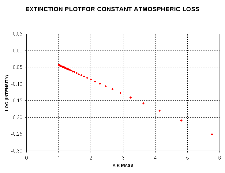
  Figure 7. Extinction plot for constant atmospheric losses. It is assumed that Log(I) outside the atmosphere is 0.00 and that each air mass has a loss of 0.1 Nepers (optical depth = 0.1).

An "extinction plot" uses log of measured intensity plotted versus air mass. If the Y-axis were simply "intensity" then perfect data plots would be curved; using Log(I) produces straight line plots, which simplifies analysis. In the above plot the modeled data has a slope, defined as dLog(I)/dm, of -0.45. The slope is a dimensionless quantity, and it should be the same for all stars (havng the same spectrum) regardless of their brightness. A slope of -0.045 corresponds to a transmission of 90% per air mass (i.e., 10 raised to the power -0.045 = 0.90). Another way of describing this situation is to state that extinction amounts to 0.11 magnitude per air mass (i.e., 2.5 * Log (0.90)). Thus, for a view where m=1 the observed star intensity is 90% of its outside the atmosphere value, at m=1 it is 81% (90% of 90%), etc. This is a typical extinction value using a V-filter under good sky conditions.

Now consider the same plot but for a linearly temporal change in atmospheric loss, as might occur when an air mass transition is in progress.

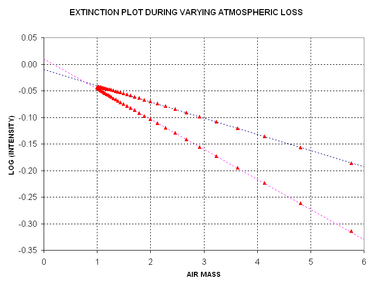
 Figure 8. Extinction plot for temporally varying atmospheric losses. The dashed lines are fitted to rising and setting portions of the measured intensity.  

I've seen this double-branched extinction plot many times during my studies of atmospheric extinction. One branch corresponds to the rising portion of data and the other corresponds to the setting portion. If intensity measurements are made during only one of the branches then a fitted slope would imply an incorrect extinction per air mass value.

Several properties of the atmosphere can contribute to temporal changes in atmospheric transmission. Sub-visible cirrus (just below the tropopause) that is present in one air mass but not its surroundings is probably the most common source. Volcanic ash can be present above the tropopause (in the lower stratosphere). Volcanoes also eject SO gas, which combines with water vapor to form sulfate aerosols, and these also will be distributed in a non-uniform manner.Water vapor in the lower troposphere is almost always undergoing change at a given site. Vapor burdens (the vertical integral from the surface to the top of the atmospehre) can vary from 1 cm to 6 cm (precipitable water vapor), and I have documented factor of two changes during a half-hour interval at a site in Pasadena, CA.  Smog is found near urban sites and the associated aerosols can contribute to large changes in atmospheric transmission. Clearly, some sites will be more prone to these atmospheric transmission changes than other sites. Coastal and urban sites will be worse, generally, but even desert sites will experience some fo the above sources of atmospheric change.

This serves to illustrate that careless observing strategies can produce extinction plots with misleading slopes, and the slopes are used to derive atmospheric extinction (Nepers of loss per air mass, or optical depth per air mass).

I can think of a couopleways to deal with an atmos[phere that is varying with time. First, restrict all observations to a small air mass range while alternating between the ROI and standard star fields. Second,  alternate observations of standard star fields that are rising and setting. If this second approach is used the two stars will exhibit discrepant slopes for the same air mass region, and this will allow a determination to be made of the temporal trend as well as an extinction value for the approximate midpoint of the observations.

I don't want to describe more details of how to process extinction plots when trends exist, for my purpose here is to simply sensitize the all-sky photometrist to a problem that is easily overlooked.

This Fundamentals section has described the reasons all-sky photometry is a challenging task, and I hope it has sensitized the prospective all-sky observer to the importance of doing it carefully. The next section will give specific observing strategies that I have found useful in performing all-sky photometry.

OBSERVING STRATEGIES 

Planning! Before every night's observing session I formulate a plan. This is especially important for all-sky photometry. Every observer will have their preferred procedure, but each procedure should address the issues raised in the previous Fundamentals section. In this section I'll present my preferred way of all-sky observing.

Assume there's just one "region of interest" (ROI) where a photometric sequence is to be determined. I use TheSky 6.0 to make a list of the ROI's elevation versus time. The preferred time to observe is when the ROI is at the highest elevation, but this is not always possible. For us poor people who mistakenly bought a German equatorial mount telescope, there's a big penalty for crossing the meridian. A dozen things have to be changed after a "meridian flip" and the data on each side of the meridian are not guaranteed to be compatible. I NEVER do all-sky photometry with my Celestron CGE-1400 using data from both sides of the meridian. In fact, I always observe on just one side of the meridian the entire night, photometry or not, and thus avoid the nuisance of all that "meridian flip" routine. (I'll never buy another GEM, never! For my diatribe against German equatorial mounts for photometry, go to http://brucegary.net/CGE/x.htm)

After deciding on the range of time (and elevation) for the ROI observations, groups of well-calibrated standard stars can be chosen. The guideline for this is to observe standard stars in such a way that they are observed throughout the same range of elevations as for the ROI. I try to include at least at least one group as close to zenith as possible and another as low in elevation as possible. In addiditon, I try to include groups of standard stars at the beginning and end of the night's observing session athat are at the same elevation, preferably near the ROI's low elevation range. This choice will be useful in assessing the existence of temporal trends.

With TheSky displaying in the "horizon" mode it is easy to see which stars are at elevations of interest. I often use the Landolt list of well-calibrated stars for my primary calibration. The Landolt list contains 1259 stars in groups that are mostly along the celestial equator, as shown in the follwoing figure.

Figure 9.  Locations of Landolt stars.  Declination [degrees] is the Y-axis and RA [hours] is the X-axis. (Note that RA shows a negative sign, due to a limitation of my spreadsheet program.)

TheSky is able to display this list of stars (with whatever symbols you like) by specifying the Landolt text file's location in the Data/SkyDatabaseManager menu. You can download this Landolt text file from LandoltTextFile. 

Since none of the Landolt stars go through my zenith I also depend on Arne Henden's set of sequences (constructed mostly for the AAVSO, I suspect). His data can be found at Arne1 and Arne2.

A third source for standard stars is the large database maintained by the AAVSO. You first have to pick a star that's in the AAVSO chart database and then download a chart for it. Not all charts are good quality, and only a few have more than just V-magnitudes, so this data source is inconvenient

Example Observation Session

To illustrate the procedure I use for all-sky photometry I will use an observing session conducted June 19, 2004 (UT). A Celestron CGE-1400 telescope was used with a SBIG ST-8XE CCD at prime focus, using a Starizona HyperStar adapter lens. Custom Scientific B, V and R photometric filters were used. All images were made with the CCD cooled to -10 C. Focus adjustments were made several times during the 3-hour observing session. When I'm using a prime focus configuration the Custom Scientific filters are not parfocal, and this required that I refocus for each filter change. I used a table of previously-determined filter focus offsets. Sky conditions were "photometric" and based on atmospheric seeing of the past few nights and the recent reliability of ClearSkyClock seeing forecasts for my site, I suspect that the seeing afforded FWHM ~ 2.3 "arc (for a Cassegrain configuration). The prime focus configuration produces a "plate scale" of 2.8 "arc/pixel, and due to slight distortions caused by an imperfect prime focus adapter lens I was able to achieve FWHM of no better than 7.5 "arc. I at least covered a large field of view, 72 x 48 'arc, using a "fast" system, f/1.86.

The purpose for the June 19, 2004 observing session was to establish a photometric sequence for a cataclysmic variable that had been recently discovered as a suspected nova. The object has a designation of 1835+25 (plus a temporary designation of VAR HER 04). This outbursting binary star is located in the constellation Hercules (about a minute of arc from the border with Lyra), at 18:39:26.2, +26:04:10. The magnitude for the June 19 observations was ~12.7.

The following figure is a screen shot of TheSky ver. 6.0 showing how two Landolt star groups and one Arne Hendon sequence (for an AAVSO blazar) were selected for use to calibrate a star field near the new nova, labeled "Nova 2004".

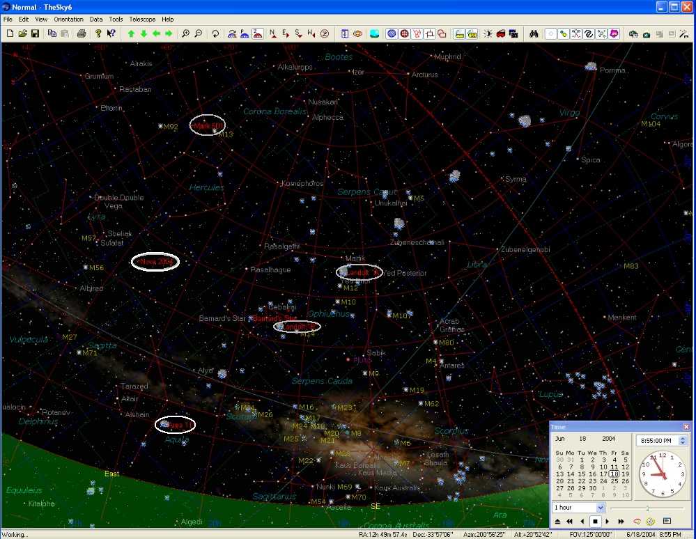
Figure 10. Resized and compressed screen shot of TheSky in horizon display mode showing the region of interest ("nova 2004", within middle-left oval), two Landolt star groups (middle-right ovals), Area 111 (lower-left oval, containing Landolt stars) and an AAVSO chart with Arne Henden calibrated stars (top-left oval). Other Landolt star groups are shown by the blue symbols. The meridian is shown by a red dashed trace from the lower-right horizontothe top-middle border. Elevation isopleths are shown by thin red traces parallel to the horizon. (The reduced size, compression and conversion to JPEG greatly degrades readability, made necessary to keep the file size reasonable.)

Other "planetarium" display programs can probably also be used to select standard stars (but the TheSky is a great deal and has all the features any CCD photometrist would want).

After selecting the groups of standard stars to be used as a primary magnitude standard an observing schedule should be decided upon. Recall the two strategies described briefly in the previous section for dealing with slowly varying extinction: 1) restrict all observations to a narrow range of elevations and alternate observations of standard star regions with the ROI, and 2) alternate observations of standard star fields that are rising and setting and determine the trend as well as an average extinction value that can be used with the ROI observations (made later, earlier or during the standard star observations).

Since my telescope is on a German equatorial mount the second option is not feasible. Therefore, I always employ the first strategy for dealing with the possibility of extinction trends during an observing session. For the observing session being used as my example I decided to start out observing the "Landolt A" group (right-most oval) and then the ROI (lower-left oval). This timing places the two targets at about the same elevation, and closely spaced in time, which means that this pairing will be unaffected by later assumptions about temporal extinction trends and extinction values. This is a conservative strategy, and it assures that something useful could be done with just the first two targets (in case of equipment problems or other show-stoppers prevented later targets from being observed). It may not have been the best strategy, but for this observing session I then observed Markarian 501 (upper-left oval), the ROI, Landolt A, and continued through that cycle until one of the targets reached the meridian, then an observation of Area 111 at a low elevation (since it rose late in the night's observing).

Notice that the first Landolt A standard stars and the Area 111 standard stars are to be made at about the same elevation and are at the beginning and end of the night's observing session. This makes them an ideal pair for assessing any trend in extinction value.

My observing plans included a list of things to do before dark. For example, review the previous observing session log notes to recall if anything anomalous occurred, review which filters are in the filter wheel (I have a SBIG "pretty picture" set and a photometric set), review the CCD settings that were last used (hardware present, flip values, image scale for proper centering), review the adequacy of the last pointing map, and determine if any telescope reconfiguration and rebalancing will be needed. For this specific observing session I had to reconfigure from Cassegrain to prime focus using the Starizona HyperStar field flattening lens, and this had to be done before dark. This also requried a rebalance and an approximate refocus using nearby mountains (so that the flat fields would be at the correct focus setting). I also had to replace some "pretty picture" filters with photometric filters. My plan had to include new flat fields shortly after sunset, for each filter, and a completely new pointing calibration (using MaxPoint). Every reconfiguration and rebalance requires a new pointing calibration. The plan called for setting the CCD cooler to a value that could be established quickly (such as +5 degC), prior to the flat field images of the zenith sky after sunset. The plan also included a sequence of targets, as well as the brightest star to be included in the analysis (needed for establishing an exposure time that does not lead to "saturation" of the brightest star). Users of MaxIm DL 4.0 will recognize some the tasks listed above. That's the hardware control and image analysis program that I use.

All pre-target items on the plan were implemented before sunset. After the flat fields were complete I cooled the CCD as far as possible. I determined that the night's CCD cooler setting would be -10 degC for the entire night, since that's as cold as I could get without exceeding a cooler (TEC) duty cycle of 90%. For all-sky photometry it's absolutely essential to use the same CCD cooler setting the entire night, and to periodically check that the cooler duty cycle is not approaching 100% (due perhaps to a warming that could be caused by sundowner winds for example).

I observed each target field with the B, V and R filters. Each filter had to be focused differently since my photometric filters are not "parfocal" when at prime focus (the pretty picture filters are parfocal). An exposure time had to be determined for use on all targets. This probably isn't necessary, but that's my current preference. A long exposure would cause saturation for the brightest stars, rendering them unuseable for photometry. I decided upon an exposure time of 10 seconds after quickly studying the first V-filter exposure of a star field with known magnitudes.

While observing I keep an "observing log" with an ball point pen.  After observations have terminated I use only a pencil to add comments based on recollections. This ink/pencil distinction can help in reconstructing what really happened months later if a re-analysis or review of the observations is made. For each exposure sequence I note such things as UT start time, object, filter, exposure time, guided (by AO-7 image stabilizer) or unguided, focuser sensor temperature (taped to the telescope tube), outside air tempreature, wind speed and direction, and sometimes my impressions of data quality as I calibrate and review images coming in "on the fly."  When a focus sequence is performed I log the focus setting and 6 FWHM readings for a sequence of focus setting valeus centered on the expected best focus position. As soon as this set is completed I plot FHWM  for the best 3 of each set of 6 FWHM readings, and do a hand fit trace to establish the best focus setting. I note what the best FWHM value is for the focus sequence, and use that as a reference to monitor drift away from best focus during later imaging in order to determine when a new focus sequenmce is needed.

On this occasion, June 19, all standard star fields and the ROI were observed successfully. Depending upon how tired I am I try to begin data analysis shortly after observations are completed. Invariably, data analysis is best done as soon after observations as possible. The memory of odd occurences and other impressions fade with time, and during analysis all these extra memories are potentially helpful.

ALL-SKY ITERATIVE PHOTOMETRY - CONCEPTS AND INITIAL SYSTEM CALIBRATION

Differential photometry with MaxIm DL can be done manually or with a photometry tool. The photometry tool is preferable because it rejects outliers in the sky reference annulus. However, for all-sky photometry the needed measurement is "intensity", and this is not recorded by the photometry tool. (If you're not using MasxIm DL and your image analysis program doesn't display intensity as you move the 3-circle pattern over the image, then buy MaxIm DL or a program that does display intensity.) Therefore, manual readings are required for each star to be included in the analysis.

It is absolutely necessary to use the same signal aperture size for ALL manual readings of intensity for an entire all-sky observing session. Small changes in the sky reference annulus are OK, as are small changes in the gap annulus - but give careful thought to the signal aperture size before starting to measure and record intensities.My suggestion is to use the fuzziest image that you're convinced you need to use and select a signal aperture radius of ~1.5 times the FWHM of a star that has a signal-to-noise ratio (SNR) within the range 50 to 300. Be certain that the FWHM is for a star that is not saturated (i.e., that has a maximum counts value less than 40,000).

Raw images should be calibrated using the appropriate dark frames. Flat frame calibration should also be applied to all images. For each field and filter and observing sequence, a median combine should be performed...

Star Intensity Readings

When making readings of intensity there is the matter of how to position the aperture circles. For bright stars (SNR > 50, for example) I use the position that yields the greatest intensity. For fainter stars I manually position the aperture circles so that brightest pixels are at the center of the signal aperture circle. Often a greater intensity reading occurs at one of more pixels away from this setting, but that is usually due to the sky reference annulus including a slightly different set of pixels and random noise can change the sky reference level depending on which pixels are included in the sky reference annulus. This effect is unimportant for bright stars, but it can dominate intensity results for faint stars.

Intensity readings are made for all Landolt (and other) standard stars, as well as a selection of stars in the ROI. These should be noted in a reduction log (using pencil). Intensity is defined to be the sum of all "extra" counts within a signal circle, where "extra" means differences with respect to the average count value within a sky referecne annulus. The sky reference annulus is separated from the signal circle (aslo called an aperture circle) by an annulus shaped gap, which allows the signal circle to be kept as small as possible while preventing the sky reference annulus from "contamination" by starlight from the star in the signal circle.

Extinction Determination

After all stars have their intensity measured for all images the next step is to determine an atmospheric extinction for each filter. Considering each filter in turn, and determine the air mass range for each field. Probably it is best to choose the field with the greatest air mass range for determining extinction, for each filter (note: it's OK to use the ROI with unknown star magnitudes for this purpose). When a star field has been chosen for determining extinction for a given filter the measured intensities should be entered into a spreadsheet program (such as Excel).

Figure 11. Extinction plot for one field of stars (the ROI) for R-filter measurements. Each intensity measurement was converted to "2.5 * LOG(Ir)" before it was plotted. The slope for each fitted straight line is -0.19 "2.5 * LOG(Ir)" units per air mass, which was the best fit.

The graph shows that one slope [having units of LOG(I) per air mass], with offsets for each star, fits all extinction plotted data. A best fit slope value can be determined by a variety of techniques. I find it useful to enter trial values for extinction, K [mag/m] or magnitude change per air mass, into a cell in the spreadsheet and note the average RMS residual fit between a least squares fit model and all measurements. Each time an extinction value is entered the spreadsheet calculates a best fit intercept for each star (using K*mav and sum of 2.5*LOG(I) /N, where N is the number of air mass obserations and mav is the average air mass; details left to the student). This "trial and error" procedure is a manual least squares solution for K, and it should be performed for each filter. Afterwards, there will be a set of K values for each filter, such as 0.25, 0.20 and 0.15 [mag/m], corresponding to the magnitude change per air mass for B, V and R filters.

Extinction Trends Evaluation

So far this procedure has not allowed for a determination of extinction trend. Since the June 19 observing date was planned to have negligible effect from extinction trends it is not necessary to evaluate it. However, for the purposes of this web page let us do this using the first and last standard star fields that were observed at about the same air mass. Since B-filter measurements experience the greatest level of extinction the B-filter data can be expected to show a greater effect than the other filter data. However, for this particular data set there are no pairs of osbervations separated by a large time span that are at the same air mass. The V-filter data comes the closest to having similar air mass measurements with a large time span separating them, so that's the data I'll analyze for an extinction trend.

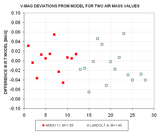
Figure 12. Deviations from extinction model that has no extinction trend for V-filter observations of Area 111 (m=1.55) and Landolt A (m=1.40) taken 1.8 hours apart.

The two sets of V-filter measurements appear to fit the same model for converting intensity, B-V color, extinction and air mass to V-magnitude. The two data groups deviate from this single extinction model by 0.012 +/- 0.030 magnitude. Taking into consideration their average airmass of 1.47, and the 1.8-hour time span separating them, the two groups of data imply an extinction trend of 0.004 +/- 0.011 [magnitude per air mass per hour]. This is statistically insignificant, and the trend, even if it were real, would be 3.0 +/- 7.6 [%/hour] decrease in the average 0.15 [magnitude/air mass] extinction value. Even if this extinction trend were real it would produce V-magnitude errors of +0.008 +/- 0.020 at one end of a 3-hour observing interval and -0.008 +/- 0.020 at the other end of the observing interval (for an average air mass of 1.33). Uncertainties at this level are small compared with the other uncertainty components, so it is legitimate to assume that extinction was not changing during this particular observing session.

Converting Intensity to Star Magnitude Using Standard Stars

It is intuitively reasonable to think that a star's measrued "intensity" (as defined above) contains information about its brightness. Consider the simplesst possible plot of this, using well-calibrated standard stars, in which Intensity is plotted versus true magnitude. The following data is from an observing session on October 15, 2004, and includes 3 Landolt areas with a total of calibrated 80 stars. 

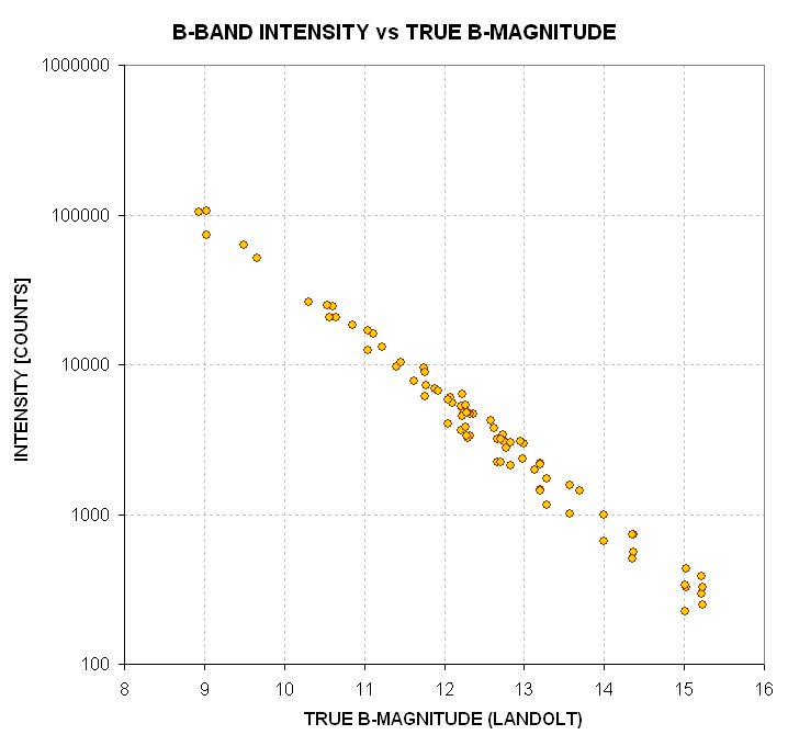
Figure 13. Measured intensity of standard stars in B-filter images for 80 Landolt stars (2004.10.15).

Indeed, the intuitive idea that measured intensity is related to true V-magnitude is borne out by this graph. The graph suggests that we should plot the LOG (to base 10) of measured intensity versus true B-magnitude. In fact, if we plot 2.5 times LOG(1/Intensity) we should have a parameter that is closely related to magnitude, subject to the same offset for all stars.

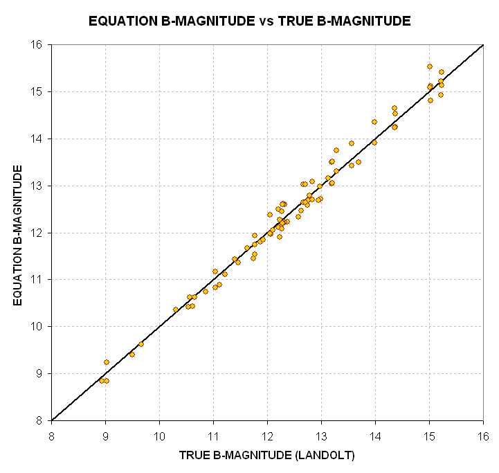
Figure 14. Plot of 2.5 * LOG(Iv) +18.9 (arbitrary offset), labeled "EQUATION B-MAG" in the graph, using the measured intensities (Ib) of standard stars in B-filter images.

Sure enough, by playing with arbitrary offsets it was possible to find an offset value (+19.8) that affords a fairly good correlation of converting "2.5 * LOG(10/Ib) plus offset" with the true B-magnitudes of the standard stars. This equation doesn't take into account the different air masses of the various images from which intensity measurements were made, nor does it take into account the different colors of the standard stars. The colors should matter since the observing system has a unique spectral response (caused by the corrector plate, prime focus adapter lens, filters and CCD response, as well as the atmosphere). Let's plot the deviations of the above measurements from the fitted line and see if these differences correlate with air mass and star color.

 

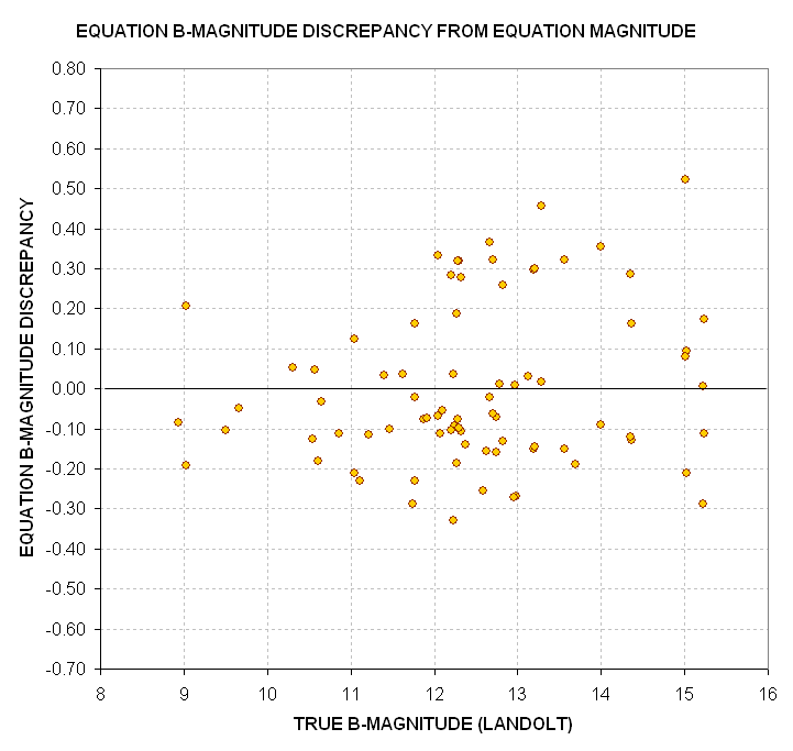
Figure 15. Discrepancies of simple "Equation B-magnitude" versus True B-magnitude for 80 Landolt standard stars.

The next question we naturally think of asking is "Are these errors correlated with air mass and star color." We also should ask if there's a statistically significant correlation with the product "air mass times star color" since a str's apparent color (entering the telescope aperture is affected by total extinction). A multiple regression analysis should show whether there is a signitificant correlation with any of these three independent variables. The answer is "yes, the errors are correlated with all three independent variables." The resultant discrepancies are much better "behaved" than those in the previous figure which ignored these three new independent variables, as the following graph shows.

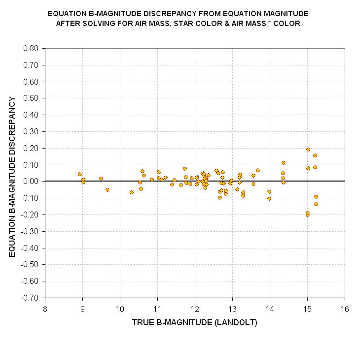
Figure 16. Discrepancies of "Equation B-magnitude" versus true B-magnitude for 80 Landolt standard stars after solution that uses the three independent variables:  air mass, star color and "air mass times star color."

The coefficients are +0.229 +/- 0.010 [magnitude per air mass], +0.090 +/- 0.051 [magnitude per B-V mag], and +0.063 +/- 0.027 [magnitude/air mass times B-V mag]. All three correlation coefficients are statistically significant. When these correlations are taken into account the simple equation becomes:

Notice that this equation uses 0.64 for a reference B-V star color; this is the median B-V value for the 1256 Landolt stars in my data base. It will be convenient to use (B-V)-0.64 as an indepenent variable in order to simplify analyses for stars with unknown B-V colors (as will be apparent below). Also notice that the LOG term has "10" in the numerator. This refers to the fact that the measurements were made with an exposure time of 10 seconds. The reciprocal of the LOG term is the ratio "Ib/10" and this ratio is merely the rate of intensity counts per second, which should be the same for all exposure times (neglecting stochastics).

In this plot the faint stars exhibit a larger scatter than the bright ones, which is to be expected from SNR (signal-to-noise ratio)  considerations.

Using all terms and coefficients derived for this B-band data leads to an improved "Equation B-magnitude" as shown in the next figure.

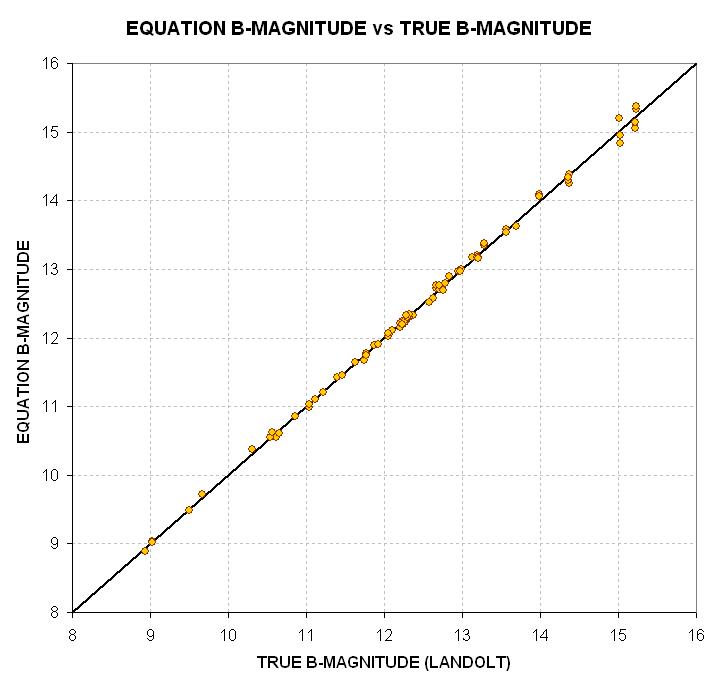
Figure 17. Equation-based B-magnitude (given in text, below) versus true B-magnitude for 80 Landolt stars. The RMS scatter for stars brighter than 15th magnitude is 0.043 magnitude.

This figure is to be compared with Fig. 14, which does not contain extinction or star color terms. Clearly, the extinction and star color are important independent variables for the task of inferring B-magnitude from measured intensity.  The final equation used for this data set is given below:

Equation B-magnitude = Cb1 + Cb2 * (2.5 * LOG(G/INTb)) + Cb3 * m + Cb4 * ((B-V) - 0.64) + Cb5 * m * ((B-V) - 0.64), where                                Eqn 4
            Cb1 = 19.31 [mag]                    related to telescope aperture, filter width & transmission, dirtiness of optics (including dew formation), signal aperture size,
            Cb2 = 1.00                                empirical multiplication factor (related to non-linearity of CCD A/D converter),
            Cb3 = -0.228 [mag/air mass]     extinction for B-filter for the specific atmospheric conditions of the observing site and date,
            Cb4 = +0.097                            related to observing system's color response (i.e., the old CCD transformation equation coefficients),
            Cb5 = +0.06                              related to product of star color and air mass,
            G = exposure time (integration gate time), seconds
            INTb = intensity using V-filter (integrated excess counts within signal aperture that exceed expected counts level based on average counts within sky reference annulus), and
            m = air mass,
            with a residual RMS of 0.043 magnitude (for the 80 standard stars brighter than magnitude 15, air mass range = 1.19 to 3.04).

Notice that Cb2 isn't necessary because it's 1.00; it is included for the occassion when stars are included in the analysis that are so bright that they begin to saturate the A/D converter in the CCD camera causing non-linearities that affect only the brightest stars.

A similar analysis performed for the V-filter data yields the following.

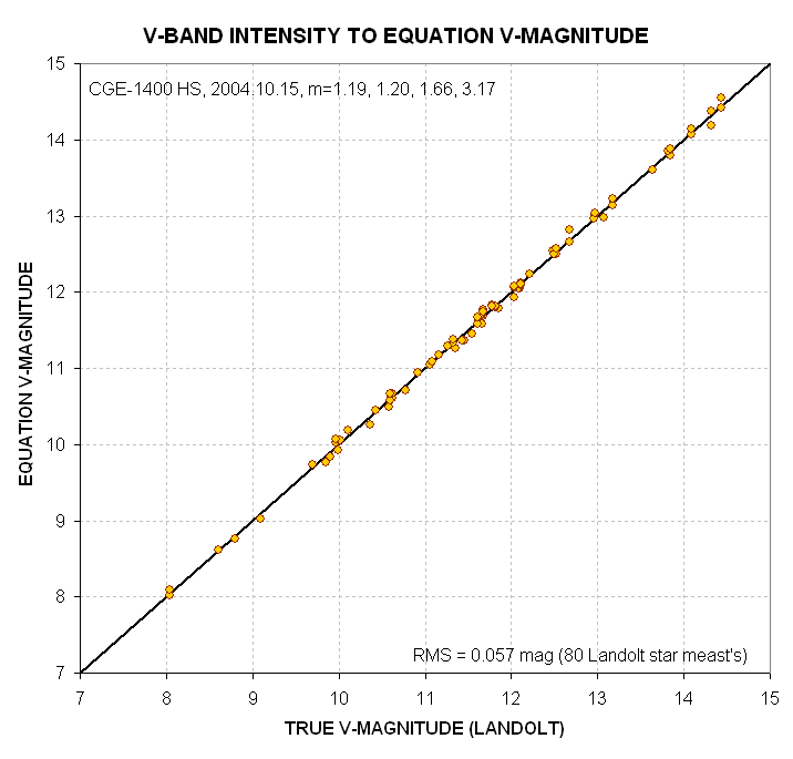
Figure 18. Equation-based V-magnitude versus true V-magnitude for 80 Landolt stars.

Predicted V-magnitude can be expressed using the following equation:

            Equation V-magnitude = Cv1 + Cv2 * 2.5 * LOG(G/INTv) +Cv3 * m + Cv4 * ((B-V) - 0.64) + Cv5 * m * ((B-V) - 0.64),                                  Eqn 5
            Cv1 = 19.68 [mag]                   related to telescope aperture, filter width & transmission, dirtiness of optics (including dew formation), signal aperture size,
            Cv2 = 1.00                               empirical multiplication factor (related to non-linearity of CCD A/D converter),
            Cv3 = -0.147 [mag/air mass]    extinction for V-filter for the specific atmospheric conditions of the observing site and date,
            Cv4 = -0.145                            related to observing system's color response (i.e., the old CCD transformation equation coefficients),
            Cv5 = +0.06                             related to product of star color and air mass,
            G = exposure time (integration gate time), seconds
            INTv = intensity using V-filter (integrated excess counts within signal aperture that exceed expected counts level based on average counts within sky reference annulus),
            with a residual RMS of 0.057 magnitude (for 79 stars and air mass range of 1.19 to 3.17)

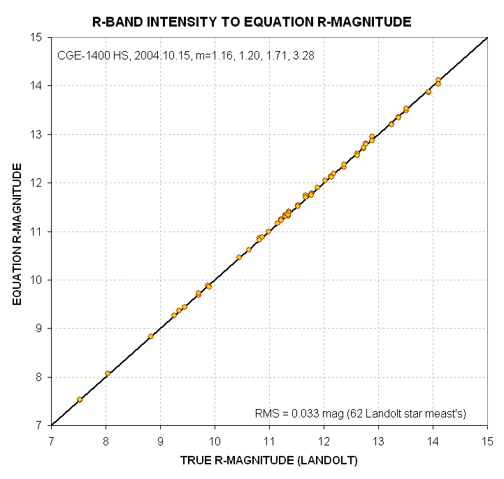
Figure 19. Equation-based R-magnitude versus true R-magnitude for 62 Landolt stars.

The R-magnitude prediction equation is:

            Equation R-magnitude = Cr1 + Cr2 * 2.5 * LOG(G/INTr) +Cr3 * m + Cr4 * ((B-V) - 0.64) + Cr5 * m * ((B-V) - 0.64),                                  Eqn 6
            Cr1 = 19.83 [mag]                   related to telescope aperture, filter width & transmission, dirtiness of optics (including dew formation), signal aperture size,
            Cr2 = 1.00                               empirical multiplication factor (related to non-linearity of CCD A/D converter),
            Cr3 = -0.100 [mag/air mass]    extinction for R-filter for the specific atmospheric conditions of the observing site and date,
            Cr4 = -0.110                           related to observing system's color response (i.e., the old CCD transformation equation coefficients),
            Cr5 = +0.02                            related to product of star color and air mass,
            G = exposure time (integration gate time), seconds
            INTr = intensity using R-filter (integrated excess counts within signal aperture that exceed expected counts level based on average counts within sky reference annulus),
            with a residual RMS of 0.033 magnitude (for 62 stars and air mass range 1.16 to 3.28)

Incidentally, it should be mentioned that unfiltered intensity measurements can be used to infer V-magnitude. Here's a graph showing how well that can work.

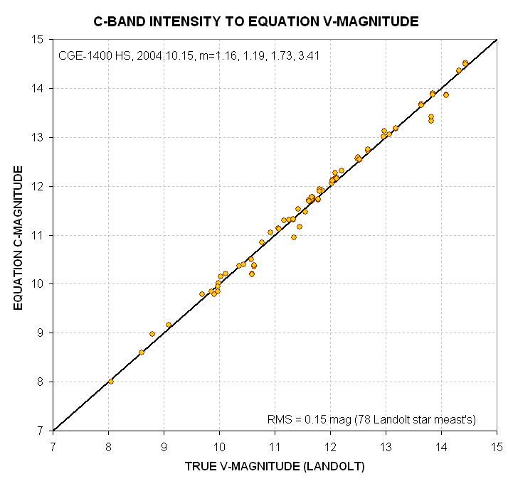
Figure 20. Equation-based V magnitude from unfiltered intensity measurements, leading to what I'm calling C-magnitude.

The equation for C-magnitude (estimated V-magnitude from unfiltered intensity measurements) is:

            Equation C-magnitude = Cu1 + Cu2 * 2.5 * LOG(G/INTu) +Cu3 * m ,                                                      Eqn 7
            Cu1 = 21.37 [mag]                   related to CCD temperature, exposure time, signal aperture size, telescope aperture, filter width & transmission,
            Cu2 = 1.00                               empirical multiplication factor (related to non-linearity of CCD A/D converter),
            Cu3 = -0.100 [mag/air mass]    extinction for clear filter (unfiltered) for the specific atmospheric conditions of the observing site and date,
            G = exposure time (integration gate time), seconds
            INTu = intensity using no filter (or "clear" filter),
            with a residual RMS of 0.15 magnitude (for 78 stars and air mass range 1.16 to 3.41)

I am surprised that the attempt to infer a V magnitude using unfiltered intensities, which I'm calling C-magnitude, works as well as this analysis of 78 Landolt stars implies that it can. Almost all of the 0.15 magnitude RMS can be attributed to not knowing the B-V star color (if that information is allowed to be used the RMS becomes 0.054 magnitude). The typical situation for trying to infer V-magnitude from unfiltered measurements is one in which no B- or V-filter observations are available, so the 0.15 magnitude RMS performance is the relevant performance number.

Iterative Procedure for Unknown Region

The previous section shows that if you know a star's magnitude you can derive it from an image - big deal! This is leading somewhere, though. The equations, above, state that once you've derived coefficients that work well for standard stars, it's possible to determine magnitudes for unknown stars from the following measured properties: intensity, air mass, and star color (B-V). But for an unknown star even though you can measure its intensity at a known air mass it doesn't have a known color index, What to do?

Iteration!

Consider the following example (and it's an extreme example since this star is unusually blue).

Star 1835+25 is a cataclysmic variable. During the June 19 observing session (with exposure times of 10 seconds) it was measured to have the following:

    06:33.5 UT   m = 1.08    INTb = 3308    SNR = 141
    05:29.6 UT   m = 1.23    INTv = 5830    SNR = 218

Let's convert these measured properties to a V-magnitude (and a B-magnitude).

We'll start by assuming B-V = 0.64, the median value for the Landolt stars . This allows us to calculate approximate B- and V-magnitudes. Using Eqns 4 and 5:

    1835+25's B-mag = 19.31 +1.00 * 2.5 * LOG(10/3308) - 0.228 * 1.08 +0.097 * (0.64 - 0.64) + 0.06 * 1.08 * (0.64 - 0.64)
    1835+25's B-mag = 12.75

    1835+25's V-mag = 19.68 +1.00 * 2.5 * LOG(10/5830) - 0.147 * 1.23 - 0.145 * (0.64 - 0.64) + 0.05 * 1.23 * (0.64 - 0.64)
    1835+25's V-mag = 12.59, so a better estimate for B-V is +0.16

    1835+25's B-mag = 19.31 +1.00 * 2.5 * LOG(10/3308) - 0.228 * 1.08 +0.097 * (0.16 - 0.64) + 0.06 * 1.08 * (0.16 - 0.64)
    1835+25's B-mag = 12.68

    1835+25's V-mag = 19.68 +1.00 * 2.5 * LOG(10/5830) - 0.147 * 1.23 - 0.145 * (0.16 - 0.64) + 0.05 * 1.23 * (0.16 - 0.64)
    1835+25's V-mag = 12.63, so now B-V = +0.05

The new B-V value departs even more from the standard star typical value, but at least it changed by only 0.05 magnitude units. Let's adopt this B-V value for the next iteration.

    1835+25's B-mag = 19.31 +1.00 * 2.5 * LOG(10/3308) - 0.228 * 1.08 +0.097 * (0.05 - 0.64) + 0.06 * 1.08 * (0.05 - 0.64)
    1835+25's B-mag = 12.66

    1835+25's V-mag = 19.68 +1.00 * 2.5 * LOG(10/5830) - 0.147 * 1.23 - 0.145 * (0.05 - 0.64) + 0.05 * 1.23 * (0.05 - 0.64)
    1835+25's V-mag = 12.64, so now B-V = +0.02

It appears that the changes in V and B-magnitudes are getting smaller each iteration, and the B-V changes are also getting smaller with each new iteration. It seems like convergence is occurring. Just one more iteration is needed (since my spreadsheet shows that no more changes occur after it), yielding:

    1835+25's B-mag = 12.65
    1835+25's V-mag = 12.64, and B-V = +0.01

The following figure is a screen capture of an Excel spreadsheet showing how an iteration (involving the above data as one of the three BV observations sets) was performed (effortlessly).

  

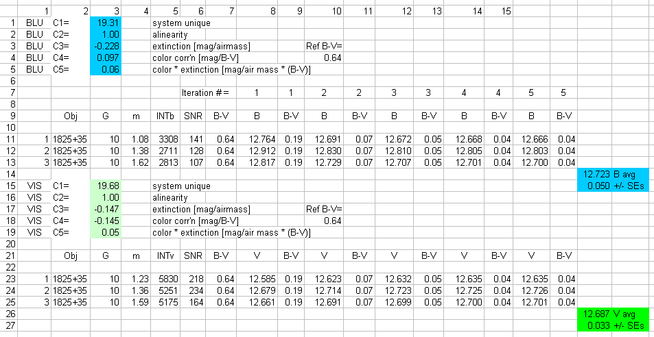
Figure 21. Screen shot of an Excel spreadsheet showing how cells containing Vand B intensity measurements for each of three data pairs were automatically calculated once values were entered for m and INTb or INTv. Rows 1 to 5 contain B-filter coefficients for converting measured B-filter image star intensity, airmass and color to B-magnitude. Rows 11 to 13 contain measured intensity for 3 B-filter images having different air mass values. Rows 15 to 25 are V-band counterparts to rows 1 to 13 for three V-filter images. The sequence of solutions for B and V-magnitudes is shown in columns 8 through 17. Convergence is apparent. SNR can be used to calculate stochastic uncertainty SEs, but so can the set of 3 measurements of the same parameter. Column 18 contains average magnitudes using the converged solutions and shows the stochastic uncertainty of the averaged magnitudes based (in this case) on the RMS scatter of column 16 values.

It is apparent that convergence is achieved after 4 iterations. Additional columns can be inserted if convergence requries it. Rows can be inserted when more than three images are available for analysis.

The following image illustrates how the analysis procedure just described can be used to create a "photometric sequence" for a star field with several candidate refernce (comparison) stars.

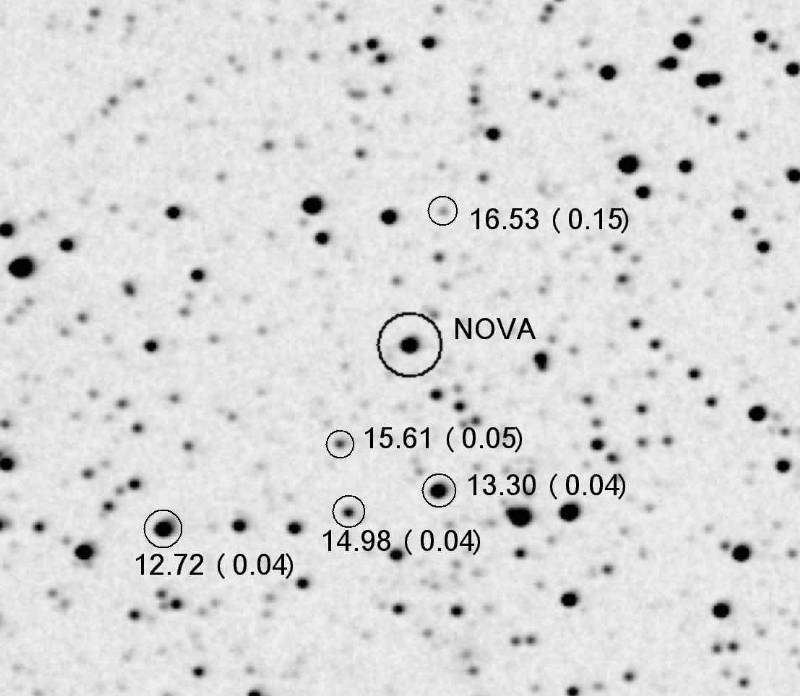
Figure 22. V-magnitudes for the nova's star field. North is up and east to the left. FOV is 24.8 x 25.1 'arc (EW & NS). FWHM resolution is ~8.5 "arc.  The nova is shown by a rectangle, and at the time of the images that were used for this average image (June 19.2 UT) the nova had a V-magnitude of 12.75.

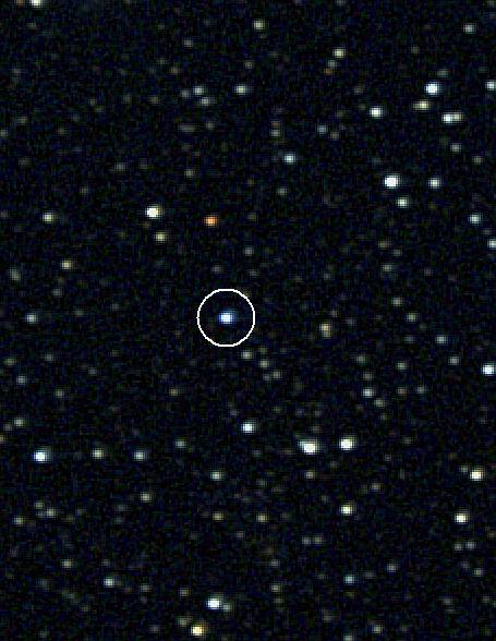
Figure 23.  This is the mysterious blue star 1835+25 (VAR HER 04). North is up and east is left for both images. The image is a RVB color image has a FOV = 10.6 x 13.9 'arc, which is a 4% areal crop of a prime focus image taken with a 14-inch Celestron telescope (prime focus, f/1.86), and the FWHM resolution is ~8.5 "arc. Notice the very red star north of 1835+25 (having B-V = +1.62, versus -0.10 for 1835+25).

SUBSEQUENT ALL-SKY OBSERVING SESSIONS

The previous section describes an initial session for calibrating an observing system. It produces values for the all-sky coefficients Cb1 to Cb5 (for the B-filter), Cv1 to Cv5 (for the V-filter), etc. Once this initial calibration has been performed it is only necessary to re-evaluate one or two coefficients per filter for subsequent all-sky photometry observations. To understand this, let's consider the "meaning" for each of the 5 all-sky coefficients, using Equation V-magnitude as an example.

    Equation V-magnitude = Cv1 + Cv2 * 2.5 * LOG(G/INTv) +Cv3 * m + Cv4 * ((B-V) - 0.64) + Cv5 * m * ((B-V) - 0.64),                                  Eqn 5

            Cv1 = 19.68 [mag]                   related to telescope aperture, filter width & transmission, dirtiness of optics (including dew formation), signal aperture size,
            Cv2 = 1.00                               empirical multiplication factor (related to non-linearity of CCD A/D converter),
            Cv3 = -0.147 [mag/air mass]    zenith extinction for V-filter for the specific atmospheric conditions of the observing site and date,
            Cv4 = -0.145                            related to observing system's color response (i.e., related to the old CCD transformation equation coefficients),
            Cv5 = +0.06                             related to product of star color and air mass,
            G = exposure time (integration gate time), seconds
            INTv = intensity using V-filter (integrated excess counts within signal aperture that exceed expected counts level based on average counts within sky reference annulus),

The value for Cv1 will be affected whenever the telesscope configuration is changed (prime focus to Cassegrain, insertion of a focal reducer, or changing from a V-filter to a G-filter). As dirt accumulates on the Cassegrain-Schmidt correction plate, or if the position of cables connected to a prime focus CCD obstruct different amounts of the aperture, Cv1 will change. When the seeing changes and a star's FWHM is too large for the user's chosen photometry signal circle aperture Cv1 may change. For example, if Cv1 was determined from Landolt star observations in a way that 100% of the point spread function (PSF) was contained within the photometry signal aperture, and if a new set of photometry analyses are performed when the seeing was worse (or with a smaller signal aperture circle), it is possible that not all of the PSF will be contained within the photometry aperture circle, and this would require the use of a different Cv1 value. Therefore, every use of Equation V-magnitude (or Equation B-magnitude, etc) should involve a solution (or quick check) for Cv1 (Cb1, etc).

Cv2 should be the same for all images since a specific CCD's non-linearity shouldn't change.

Cv3 is the atmosphere's zenith extinction for the V-band filter, and it is necessary to re-evaluate this parameter only when the Landolt stars and the region of interest (ROI) are at different elevations (air masses). The meaning of "different" in this case depends on desired accuracy. For example, if zenith extinction can be counted on to vary within the range 0.14 to 0.15 whenever the sky is clear (and clean), then an air mass difference of 0.20 will lead to differences in line-of-sight extinction of 0.030 magnitude. If this is acceptable, then provided air mass for the Landolt area and region of interest can be kept the same to within 0.20 then it is not necvessary to evaluate the night's zenith extinction.

Cv4 is related to the telescope system's unique color response, and provided the telescope configuration doesn't change (prime focus versus Cassegrain, for example) it should be safe to adopt the value derived from the all-sky coefficient evaluation exercise.

Cv5 should undergo a change only when the atmosphere undergoes a large change in zenith extinction (in which case the sky is not of "photometric quality"). This term is unrelated to an observer's hardware (to first order), so unless it shouldn't be adjusted.

Therefore, whenever a Landolt area can be found at approximately the same elevation angle as the ROI the only coefficient needing re-evaluation is Cv1.When the Landolt area is more than 0.1 or 0.2 air masses away from the ROI then two Lanoldt areas at different air masses will have to be observed to allow evaluation of zenith extinction. If there is reason to believe that zenith extinction is changing with time then another Landolt area will have to be observed (separated as much as possible in time) that is at the same approximate air mass as one of the other Landolt areas.

The following figure illustrates how a spreadsheet can be used to easily convert measured intensity to color-corrected magnitude using a V-filter image after a one-time observing system initial all-sky calibration.

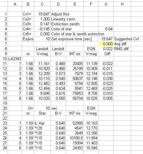
Figure 23. Example of an Excel spreadsheet section used for all-sky photometry for converting measured V-band "intensity" to V-magnitude (once an initial coefficient evaluation has been performed). Coefficients Cv2 through Cv5 are from the initial all-sky analysis. Cv1 is adjusted by the user so that Landolt stars (rows 11 to 18) differ from their known V-magnitudes with an average (cell G7, yellow) that is close to zero. The unknown stars (rows 23 to 28) are initially assumed to have a B-V color of 0.64, and when their air mass and measured intensities are entered into the spreadsheet their equation V-magnitudes are automatically calculated (cells F23 to F28).

This figure depicts an example in which the Landolt star field at RA = 23:43 was observed, and later a region near IL Aqr was observed for the purpose of establishing a photometric sequence for stars close to the variable IL Aqr. Only Cv1 was adjusted to achieve agreement (for this observing night) between the Landolt star Equation V-magnitudes and their known V magnitudes. In this example the Landolt area and ROI have air mass values that are approximately the same, and it is not necessary to evaluate zenith extinction.

The same procedure just described for V-filter measurements should be performed for B-filter measurements inorder to refine the B-V star color assumption. An iterative process is used to arrive at a stable solution for both V- and B-magnitudes, similar to that decribed for Fig. 21.

For those occasions that Landolt air mass values differ significantly from the ROI air mass it will be necessary to include observations of an additional Landolt area at a quite different air mass so that the zenith extinction parameter Cv3 can be adjusted. Performing a least squares (LS) solution with a spreadsheet is quite simple when only two independent variables are involved. You simply adjust one parameter to achieve minimum RMS, then change the other independent variable and repeat the RMS minimizing process. Practice helps, as I have determined a global LS solution for as many as 4 independent variables manually with a spreadsheet.

If zenith extinction varies with time, and if the Landolt areas and ROI can't be observed closely in time, then I leave it to the reader to figure out how to deal with this situation.

DIFFERENTIAL PHOTOMETRY ITERATIVE PROCEDURE (DPIP)

This section describes a method I have devised for differential photometry that does not explicitly employ "CCD transformation equations" nor does it require a special observing session using a standard field of well-calibtrated stars (such as exist in M67). I call it Differential Photometry Iterative Procedure (DPIP). This procedure is extremely easy to perform for observers who have done the All-Sky Iterative Photometry "initial calibration," described in the section before the last one (i.e., at the internal link ASIP). However, for those who do not want to do the All-Sky Iterative Photometry initial calibration, and this probably means just about everybody, there is a simple way to evaluate the coefficients needed for differential photometry using DPIP. In order to understand which coefficients are required for DPIP let's begin by reviewing the complete equation for All-Sky Iterative Photometry. Let's use the Equation V-magnitude terms, one at a time, to understand their meaning for this new situation.

            Cv1 = 19.68 [mag]                   related to telescope aperture, filter width & transmission, dirtiness of optics (including dew formation), signal aperture size,
            Cv2 = 1.00                               empirical multiplication factor (related to non-linearity of CCD A/D converter),
            Cv3 = -0.147 [mag/air mass]    zenith extinction for V-filter for the specific atmospheric conditions of the observing site and date,
            Cv4 = -0.145                            related to observing system's color response (i.e., related to the old CCD transformation equation coefficients),
            Cv5 = +0.06                             related to product of star color and air mass,
            G = exposure time (integration gate time), seconds
            INTv = intensity using V-filter (integrated excess counts within signal aperture that exceed expected counts level based on average counts within sky reference annulus),

Cv1 will have to be adjusted, even for differential photometry, since there is the possibility of dirt, or dew, or some other obstruction interfering with photons entering and passing through the optics and reaching the CCD.

Cv3 is the atmosphere's zenith extinction for the V-band filter, and since we are now dealing with differential photometry there is no need to re-evaluate it. Changing Cv3 will have no effect upon the Equation V-magnitude calculation anyway, so any old value for this coefficient is equally acceptable.

Cv4 is related to the telescope system's unique color response, and provided the telescope configuration doesn't change (prime focus versus Cassegrain, for example) it should be safe to adopt the value derived from the all-sky coefficient evaluation exercise. To evaluate Cv4 it is necessary to obtain an image with calibrated stars having a range of B-V colors. If this coefficient has not yet been evaluated, don't worry, we'll do it as a part of DPIP.

Cv5 should change only when the atmosphere undergoes a large change in zenith extinction. This term is unrelated to an observer's hardware (to first order), so it shouldn't be adjusted. If it is ignored, errors are typically ~ 0.01 magnitude, but for very red or blue stars the error could be as high as 0.05 magnitude. Because of this possibility I suggest including this term with an adopted coefficient value for all spreadsheet iterations.

The conclusion from the foregoing is that only Cv1 and Cv4 (and for very red or blue stars, Cv5) are needed for differential photometry. Cv1 is easily adjusted using the V magnitudes of the reference ("comp") stars in the target image's FOV. Cv4 contains information about the unique color response of the observing system (filters, CCD spectral response, etc) and is analogous to the T_v term used in the standard CCD transformation equations. It must be evaluated using a field of stars with known B-V. If the chart contains reference stars with a wide range of B-V then the image containing the target star can be used for evaluating Cv4.

The following figure can be used to show how differential photometry can be performed using the chart reference ("comp") stars to evaluate Cv1 and Cv4.

Figure 24. Example of an Excel spreadsheet section used for a differential photometry first iterative step for converting measured V-band "intensity" to V-magnitude. All measurements of V-filter intensity are made from the same image and are entered in cells E11 to E18 for the 8 known reference ("comp") stars (for this example I am using Landolt stars from a region near RA = 23:43) and cells E23 to E28 for 6 "unknown" stars whose V-magnitude is desired (for this example I'm using nearby Landolt stars as pretend unknowns, in order to assess accuracy of the final result). Coefficients Cv1 and Cv4 (in cells colored green) are adjusted by the user to achieve zero average magnitude error for the reference star Equation V-magnitudes with respect to their true Landolt V-magnitudes and to achieve minimum RMS deviation of Equation V-magnitudes from their Landolt values (using the yellow cells to show average and RMS difference).  The other Cv coefficients have either adopted values (Cv2 and Cv5) or the value doesn't matter (Cv3). When the user achieves a solution for the green cell coefficietns the Equation V-magnitudes for the unknown stars are automatically calculated (using B-V of 0.64 for this first iteration). The blue block of cells show information that is not normally available but for this example is available since my "unknown" stars are Landolt stars near the other Landolt stars used as reference stars.

DPIP FOR DUMMIES

In case you want to skip all the concepts, theory and explanations in the preceding section, and just want to try out my Differential Photometry Iterative Procedure (DPIP), this section is for you.

Download the Excel spreadsheet located at DPIP.XLS.

Figure 25. This is what you'll see when you open the Excel spreadsheet DPIP.XLS. It has sample entries for coefficients (top section), standard ("comp") star information (middle section), and unknown star information (lower section). The text explains how this spreadsheet can be used to iterate a solution for B- and V-magnitudes for the unknown stars.

Begin with one B-filter image and one V-filter image of the same star field containing calibrated reference ("comp") stars. Measure "intensity" for the reference and unknown stars. If necessary, insert rows or delete rows to accomodate your number of reference and unknown stars. Enter the exposure time for the B-band image at cell C5, and likewise for the V-band image in cell K5. Below these cells are the air mass values for the B- and V-band images; enter them in those cells. Enter the reference star known magnitudes for B and V (cells C11..C18 and K11..K18 in this example). Enter the reference star known B-V values in the B-band section (cells D11..D18 for this example); they will be copied automatically to the V-band section. Enter the measured intensities for the B-band and V-band images (cells E11..E18 for B, and cells M11..M18 for V, for this example). Enter the measured intensities for the unknown stars (cells E22..E27 for B and M22..M27 for V, for this example). The equation magnitudes for B and V will be automatically calculated (cells F11..F18 for B, cells N11..N18 fo V). These will differ from the known B and V magnitudes because the green cell parameter values have not yet been adjusted. Note the suggested Cb1 and Cv1 values in cells G6 and O6. Enter these values in the corresponding green cells (and note that the "Avg diff" yellow cells will become zero). Now, adjust green cell C3 for minimum "RMS diff" (yellow cell G8).  Do the same for green cell K3 and yellow cell O8. You're done with the first iteration! Note that the unknown stars now have approximately correct magnitudes (cells F22..F27 and N22..N27). We need to use these magnitudes to refine their B-V values. For this first iteration we assumed they had B-V = 0.64. Note the suggested B-V values in cells P22..P27. Copy the values of these cells to D22..D27 (i.e., highlight P22..P27, Edit/Copy, then place cursor at D22, Edit/Special Paste/Values/Enter). Repeat the last B-V refinement procedure until there are no changes in cell values.

That's it. You've just used DPIP to perform a solution for B and V magnitudes using a chart's "comp" stars to 1) calibrate your telescope system's color response (a quick version of that annual M67 transformation calibration), 2) adjust your zero-point offset using several comp stars (better than using just one comp star), 3) applied a correction for a second-order term that usually is only done by the professionals (the star color times air mass times zenith extinction, which affects the color of the star at your telescope aperture), and 4) prepared your spreadsheet coefficients for doing a "poor man's all-sky photometric analysis." This last point just means that you can now take an image of any unknown (uncalibrated) star field (made with the same telescope configuration) and convert measured intensity to magnitude. The exposure time can be different, and so can the air mass and CCD cooler temperature. This assumes your site's zenith extinction is approximately the same as the entries (C2 and K2), which you should probably ascertain with a special observing session.

Since most charts avoid using comp stars with widely different B-V values it's probably a good idea to observe M67, or a Landolt area with many stars that will fit withinyour CCD's FOV, and once and for all establish values for the Cb4 and Cv4 parameters. Once these have been established they should remain constant until you change the telescope configuration. When you have a good set of values for these parameters then you shouldn't solve for them when performing DPIP; instead, just solve for Cb1 and Cv1. This will make the DPIP process even simpler.

Closing Comment

As an aside, I want to say that the standard procedure suggested for use by AAVSO members is to convert apparent magnitude to true magnitude using "CCD Transformation Equations" with a set of CCD Transformation Equation Coefficients (TEC) determined once or twice per year. This procedure has the limitation that a TEC set established under one atmospheric extinction condition and one range of air mass values (and one telescope configuration) cannot be expected to perform well under different atmospheric extinction conditions and different air mass situations (and different telescope configurations). Professional astronomers employ a rigorous but more complicated set of transformation equations that explicitly take into account extinction. The procedure I am using overcomes the limitations of the simpler transformation equations without the complication of the rigorous transformation equations.

To illustrate that DPIP is simpler and more intuitive, consider the form of the CCD transformation equations:

    (V_s - R_s) = (V_c - R_c) + T_vr * [(v_s - r_s) - (v_c - r_c)]
    V_s = v_s + (V_c - v_c) + T_v * [(V_s - R_s) - (V_c - R_c)], using the solution for (V_s - R_s) in the above line
    R_s = V_s - (V_s - R_s), using V_s from the line above, and (V_s - R_s) from the first line
    B_s = V_s + (B_c - V_c) +  T_bv * [(b_s - v_s) - (b_c - v_c)]

where:

    V_c = known V-band magnitude of comparison star,
    R_c = known R-band magnitude of comparison star_,

    v_s = instrumental (i.e., measured and uncorrected) V-band magnitude of star of interest,
    v_c = instrumental V-band magnitude of known comparison star,

    r_s = instrumental R-band magnitude of star of interest,
    r_c = instrumental R-band magnitude of comparison star,

assuming the following coefficient definitions (unique to an observing system and usually unchanging):

    Tv = slope of (V-v) plotted versus (V-R)
    Tvr = reciprocal of slope of (v-r) plotted versus (V-R)
    Tbv = reciprocal of slope of (b-v) plotted versus (B-V)

No wonder many observers (including myself) are intimidated by the prospect of transforming instrumental magnitude differences to corrected magnitude differences without introducing errors.If you're still unconvinced about the merits of the iterative all-sky photometric procedure described on this web page, then you are welcome to continue using CCD tranformation equations, which I derive and explain at TEC. Even though I have derived the CCD transformation equations from essentially first principles (so presumably I understand them) I find them cumbersome and prone to error during their implementation. I think the reason they are prone to error is that they are not "intuitive" - so if you make a mistake somewhere in the procedure you're unlikely to realize it. But, "to each his own."

Return to Bruce's AstroPhotos

This site opened:  June 20, 2004.  Last Update:  March 31, 2006