SME, Simple Magnitude Equations

When I derived the CCD Transformation Equations as a self-assigned exercise a few years ago (described at http://reductionism.net.seanic.net/CCD_TE/cte.html) it just seemed that there should be a simpler way to convert measurements of star flux in a CCD image to a standard magnitude. The CCD Transformation Equations recommended by AAVSO were not only complicated, they were a subset of the complete equation set used by professionals, and the subset ignored air mass effects. This meant that the subset results were less accurate (at the 0.05 magnitude level). During the past year I have been evaluating a simplified procedure which retains the air mass and star color correction terms. I call it "simplified magnitude equation photometry," or SME photometry.

There are several variants of SME photometry, corresponding to whether the star field has some calibrated stars in the image, whether one filter or many filters are used, and whether a Landolt star field is observed. These various SME photometry procedures are more intuitive, and they provide understandable feedback to the user. One of these feedbacks which I now appreciate as essential is the ability to view a plot to identify "outlier" standard stars. These outliers can be produced when a standard star is unsuitable because it's in fact a variable, or it's a close double that wasn't noted by the user, or it was too close to the edge of the FOV where flat field errors were severe - all of which I've encountered. Perhaps more important, SME photometry is less likely to produce erroneous results due to user book-keeping mistakes that go undetected.

The SME photometry procedures range from all-sky (yielding accuracies of ~0.03 magnitude) to "lazy all-sky" (with accuracies of ~0.10 magnitude). This last one may sound poor, but it is adequate for most asteroid observers, and it is very quick. It's so simple that I frequently perform it using a hand caclulator while observing.

I have evaluated each of the SME photometry procedures by repeatedly observing standard star fields and treating them as if they were uncalibrated. This allowed me to compare derived magnitudes with "truth." I conclude with the following empirical performances when using various versions of the SME photometry procedures (in order of easiest to hardest):

While developing and refining the simplified procedure I kept asking myself why it hadn't been developed and adopted long ago. My tentative answer is that it relies upon personal computers with spreadsheets, which were not in common use until the last decade. It may be true that the simplified procedure demands too much "conceptual understanding" from the user, and I reluctantly acknowledge that an automated implementation of it could be developed (a program that relieves the user of some of the tedious though enlightening phases). I am not an enthusiast of using programs someone else has written, since only the programmer knows the program's strengths and weaknesses. In addition, I prefer to "wallow in dirty data" to get a good "feeling" for the information content of the measurements and what they are capable of conveying and what they shouldn't be counted on to convey. I reluctantly warn that anyone who hates spreadsheets should not bother reading this web page. Maybe that's the explanation for SME photometry having not been presented to the photometry community before now, since anyone considering promoting it knows that many CCD observers hate spreadhseets.

I believe in reliance upon concepts for solving problems, as opposed to being given a set of procedures to follow on blind faith. Therefore, this web page takes care to present the concepts instead of simply listing a set of procedure to be memorized. I also like presenting concepts using the simplest approximation first, then refining it by adding the next level of approximation. The person who doesn't care about underlying concepts should probably consider abandoning this web page, because blind faith always leads to disaster. For those who are merely impatient, who promise to return to this web page after sampling my examples web page, I invite you to quickly look over QuickStartExamples to see these SME photometry procedures demonstrated with real observational data.

If you're new to photometry, and you'd like to learn why so much effort is needed to produce standard magnitudes, and you're intereseted in the underlying physics of why the entire photometry subject is so complicated, you might want to review the following web page: all-sky photometry basics. That web page is slightly dated, as it is a year old and has evolved into this web page. Then here's my ultimate all-sky photometry web page, meant for the really serious amateur: Serious All-Sky Photometry Tutorial (0.025 mag SE) I think it's the best procedure for the really serious amateur, starting with a slow-paced intro but gradually rising to the formidable.

Just one more caveat before letting you loose with the following material. I believe that 90% of what people say and believe is absurdly flawed, and even though I proudly proclaim that only 50% of my utterences are wrong, I advize the reader to remain skeptical of everyting on this web page. This is especially true during the early phases of it. Only after Arne has endorsed it, if he ever does, will you be safe in assuming that it is not seriously flawed.

For every telescope/filter/CCD system there is a simple relationship between a star's flux and its magnitude. Let's begin with two simplifying assumptions: 1) there is no atmosphere, and 2) by some fortunate circumstance the telescope system is constructed so that its spectral response perfectly matches the response corresponding to the standard magnitude system. For these assumptions the following relation would exist:

where V is the V-band magnitude, Z is a zero-shift constant for the telescope system, F is the star's flux, g is the exposure time (i.e., "gate time"), and LOG is a 10-based logarithm. The term "flux" refers to the sum of counts within an aperture that includes all of the star's light minus the sum of counts that would be expected if the star were not present (based on the average sky background level). If the photometry aperture is chosen to be small (in order to maximize SNR), then F = F' / f, where F' is the flux measured using a too-small aperture and "f" is the ratio of counts using the same aperture to the counts from use of a large aperture (and "f" is established from measurements of a bright star in the same image). When I process an image of a very faint object my aperture is usually chosen so that f is in the range 0.95 to 0.98. Note that by dividing "F" by "g" we are taking the logarithm of the rate at which counts are accumulating on the CCD attributable to the star of interest and this renders the equation appropriate for any exposure time. The term Z most strongly depends on the aperture, filter and CCD characteristics, although it will change slowly as dust accumulates on the SCT corrector plate (or the mirror coating degrades on an open tube telescope).

where K [magnitudes/air mass] is the atmosphere's zenith extinction coefficient and m = air mass. (Apologies for using m for air mass, instead of the customary X symbol; I come from the atmospheric sciences where we use m.)

Consider a telescope/CCD system with the following values for the V-magnitude equation constants:

Let's consider the power of this equation. Suppose an interesting star is discovered and there aren't any charts for it, but we have a CCD image that begs for analysis to get the star's V-band magnitude. Assume we measured the star's flux to be 10,000 counts on an image with an exposure time of 100 seconds, taken at an air mass value of 2.0. What can we say about the star's magnitude? Well, the calculation is so simple we can almost "do it in our head." V = 19.54 -2.5 * LOG ( 100) -0.14 * 2.0 -0.09 * C. We don't know star color yet, so we'll start by assuming it's a typical star, with color C = 0 (that's why I defined C the way I did; more on this later). This means that for now the last term can be dropped. We then have V = 19.54 -2.5 * 2 - 0.28 = 14.26.

Since a measurement is not a measurement unless it also has an uncertainty assigned to it, we need to propogate errors and learn how accurate this magnitude is likely to be. There are two components to accuracy: 1) noise-related "stochastic" uncertainty (SEs), and 2) estimated systematic calibration errors (SEc). The first one is simple to calculate, since usually it is merely 1/SNR. If our star flux (10,000 counts) has SNR = 100, then SEs = 0.01 magnitude. Systematic uncertainties due to calibration errors (SEc) are difficult to estimate (I use the term "estimate" on purpose). As I'll describe below, it is possible to assign uncertainties for each of the constants in the above equation. For example, the constants given above are for my system at one stage of its calibration, and I have reasons for adopting 19.54 +/- 0.02, 0.14 +/- 0.01 and 0.09 +/- 0.01. If C = 0.0 +/- 0.4, then we can propogate errors to arrive at V = 14.26 +/- 0.04.

How could we achieve such an apparently good result without the fuss of laborious all-sky calibrations or CCD Transformation Equations? The answer is that we in fact did do the all-sky calibration, but it was done maybe months ago when we established values for the constants in the magnitude equation. We're just avoiding doing an all-sky calibration every night we observe by assuming that nothing about our telescope configuration has changed from the time we calibrated it. And as for CCD Transformation Equations, we haven't done them yet given that we assumed a star color instead of deriving it. But now it's time to demonstrate how easy it is to derive the star's color, the paramter C.

Suppose we have a 100-second R-filter exposure at m = 2.0 from which we measure a star flux F = 22,000 counts. Assuming C = 0 for the moment, we calculate R = 13.67. We can now test our assumption that C = 0. We have a tentative V-R = 0.59. This corresponds to C = 0.28 (recalling that C = V - R - 0.31), and this value for C differs from our assumed C = 0.00. Let's repeat the V and R calculations using C = 0.28. Doing this yields V = 14.21 and R = 13.29. This corresponds to C = 0.28. One more iteration yields the same V = 14.20 and R = 13.58 and C = 0.30 (note that round-off errors are present). No more iterations are necessary since we've achieved convergence with just three iterations.

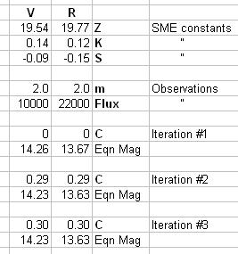
Figure 1. Spreadsheet showing 3 iterations for converting V and R flux measurements to V and R magnitudes. The final iteration is self-consistent with the star color term in the magnitude equations.

This example shows that anyone with a calibrated telescope system can make their own star chart sequences without having to observe Landolt areas (at many air mass values). This can be done using just two images of the uncalibrated star field, preferably using V and R filters (although any two filters will work).

The same spreadsheet can be used to propogate errors, both stochastic and systematic, using SNR and adopted uncertaintis for the "SME constants." When this is done the star color uncertainty component is reduced and we get the following results for this example: V = 14.23 +/- 0.04 and R = 13.63 +/- 0.04. In this particular example the solution change produced by iterating was small, and the estimated accuaracy improvement was also small, but for very red or very blue stars the changes would be larger and the accuracy improvement would be more dramatic.

I have chosen to define star color using V-R-0.31 instead of B-V for a couple reasons.

First, I prefer V-R because for a typical amateur telescope system R is ~70 times easier to measure than B! This dramatic ratio is due to the fact that a typical star has 8.3 times more flux at R than B, and since observing time for a given SNR is proportional to the square of flux ratio it takes ~70 times as long to measure a typical star with a B filter than the R filter (to the same SNR). Second, a typical star has V-R ~ 0.3, so using a parameter in which ~0.3 is subtracted from V-R means that when you're dealing with a star of unknown color you can merely delete the term (or set it to zero) and proceed to a "best current information" solution.

V-R colors are highly correlated with B-V colors for normal stars. It is therefore possible to use a converting equation when dealing with standard stars that have only B and V magnitude, which is the case for most Landolt stars. I find that V-R = 0.01 + 0.57 * (B-V) does an adequate job of converting from one color to the other. To see a graph showing how good this converting equation is click on V-R vs B-V. Since ~3/4 of the Landolt stars have only B and V magnitudes, I have adopted this conversion routine for all Landolt stars. It shouldn't matter which of the following star color equations is used:

The typical discrepancy between star color derived the two ways is <0.02, and this produces a negligible contribution to the final accuracy uncertainty when using SME procedures. Highly reddened stars can have errors of ~0.10 magnitude, but even this error propogates to small errors (for amateur work) in the SME magnitude solution.

and for unfiltered observations we can even define a new magnitude equation for estimating either V or R magnitudes:

(11) Cv = Zcv - 2.5 * LOG ( Fc / g ) - Kcv * m + Sc * C (for estimating V-magnitude)

(12) Cr = Zcr - 2.5 * LOG ( Fc / g ) - Kcr * m + Sc * C (for estimating R-magnitude)

Note that an unfiltered flux contains more information about R than about V, since about twice as many R photons are registered than V photons for a typical amateur telescope system. Therefore we should expect better performance for Cr than Cv. Asteroid observers who emphasize astrometry over photometry usually observe unfiltered so they can do a better job of estimating R-magnitude than V-magnitude, and they might want to consider using the Cr equation.

For a calibrated telescope/filter/CCD system there is a simple relationship between a star's flux and its magnitude. For example, for my 14-inch Celestron the following relations exist:

Figure 2. Simplified magnitude equations for a 14-inch telescope (Celestron CGE-1400), Custom Scientific filters, Celestron f/7 focal reducer and SBIG ST-8XE CCD, located at a 4600-foot altitude site in Southern Arizona. The last two equations are for converting unfiltered (Clear filter) fluxes to V and R equivalent magnitudes. The symbol "C" is star color, defined in the text.

The coefficients in the figure are for one telescope system, and have been determined by a process to be explained in a later section. The constants (for Zj, Kj and Sj, where j represents a filter choice) are stable from night to night, for many months at a time, and they are unaffected by the CCD cooler setting. The zero-shift constant can change if a different amount of dust is present on the mirror of an open tube telescope or corrector plate for a Schmidt-Cassegrain telescope. If the mirror loses reflectivity with time this constant will also drift. If the observing site exhibits a seasonal variation for zenith atmospheric extinction then small adjustments to the zenith extinction coefficient will have to be made (solved for). If thin cirrus clouds are present, or volcanic ash is present in the stratosphere (smoothly distributed horizontally), the zenith extinction value will have to be solved for independent of any concerns about mirror reflectivy changes and corrector plate dust accumulation. The star color sensitivity coefficients shouldn't change, unless you add or remove a focal reducer (for example), but if they have not been determined well from previous observations of calibrated star fields then they are candidates for easy solution each night.

Consider a calibrated telescope system with a simple magniutde equation like the following:

where Fv = V-band star flux (corrected for any small aperture effects), g = exposure time [seconds], m = air mass, and star color C = 0.57 * (B-V) - 0.30 or C = V - R - 0.31 (either version is OK).

On the right side of the equation everything is either known or measured, except maybe star color, C. On those occasions when C is not known, an iterative process can be used to determine it. This is done by first assuming that C =0 (which is true for typical stars with V-R = 0.3, or B-V = 0.5), then calculating first iteration estimates for V and R, where R-band observations are processed using an equation similar to (1), as illustrated here for my telescope:

After the initial iteration, producing V and R estimates, these new V and R values are used as input for a second iteration.Usually, only two or three iterations are necessary to achieve a stable solution.

There is nothing "incestuous" about this procedure. Only one pair of values for V and R will produce internal consistency.

The SME iteration procedure just described can be used when images of the region of interest (ROI) have been made using two filters (at the same approximate air mass). Notice that we did not need observations of Landolt star fields. I refer to this procedure as "Medium Quality All-Sky SME Photometry." This SME procedure should have an accuracy of ~ 0.05 magnitude.

An improvement over the preceding procedure would be to observe Landolt areas on the same night as the ROI. I usually observe a high air mass (m = 2.5 to 3.0), low air mass (m ~ 1.20) and a same air mass (as the ROI) set of Landolt areas each evening. The high and low air mass Landolt areas are most useful for refining the night's zenith extinction coefficient, the Kj parameters. All three landolt areas can be used to refine the system's sensitivity to star color, the Sj parameters (as demonstrated on the companion web page). With a sufficient number of stars (such as 20 or 30) it is even possible to establish a value for the "air mass times star color" coefficient. If you're constrained for observing time there's small loss in omitting the high and low air mass Landolt areas, provided you are confident of most of the SME constants and coefficients.

Not all Landolt areas are created equal. Some have more 4-colr information than others. Some are more spread out which is not useful for small CCD field of views. My favorite Landolt area is at 09:56:38 and -00:29:00 (which I refer to as LA0956). I can fit into my FOV (24 x 16 'arc) 15 stars with BVRI magnitudes.

The QuickStartExamples web page demonstrates the concepts of this SME procedure.

Some of the SME constants and coefficients can be verified using calibrated "photometric sequence stars" when they exist for a chart for the ROI. If you have only one image (i.e., one filter), you can refine Zj and maybe also Sj for the filter j that was used. It is not important to verify Kj since all stars are at the same air mass. The only effect of using a better Kj is to cause a small compensating change in Zj, with no change in the derived star magnitude (a wide range of compatible Zj and Kj pairs will give the same magnitude result for the object of interest). Thus, only one of these parameters needs to be adjusted, preferably Zj, when a chart with a photometric sequence is used. Chart sequences too often have a selection of "comp stars" with the same approximate color, and a wide range of brightness variation. This is good for visual observers, but it's bad for CCD observers. Some day the AAVSO will allow users to make their own chart from an AAVSO data base that contains all kinds of stars in the available photometric sequence. When this option is available (later in 2005, let's hope), the CCD user who employs SME procedures will choose as many stars as possible for "reference stars" and hopefully they will exhibit a wide range of star colors. For calibrating the SME parameters it is not necessary to have a large range of reference star brightnesses, so the best choice is only bright stars (well, stars in the V-magnitude range 10 to 14).

Incidentally, I distinguish between the terms "comparison star" and "reference star." Comps are for visual observers, and a set of them should span a large range of magnitudes with a uniform magnitude spacing, and they should all have typical colors, such as B-V = 0.5, or V-R = 0.3). The term "reference star" refers to a set of stars with a wide rnage of colors and no regard for including faint ones. The CCD observer usually performs "ensemble photometry" so the more stars the better. Ensemble photometry means that many reference stars are used to establish a calibration for all "objects" and "check stars." Ensemble photometry reduces the stochastic and some systematic error uncertainties, and there's no excuse for not using it. An additional benefit of ensemble photometry is that text files of the results of this photometry can be imported to a spreadsheet and plots can be made of RMS versus star magnitude, which in turn can be used to predict an expected SE uncertainty for an object once its magnitude is known.

When a chart with a good set of photometric sequence of stars is available for use as reference stars plots can be made of discrepancy versus star color. If a pattern with a slope exists, this means the Sj term needs refinement and it is a simple matter to determine a refined Sj value. This is demonstrated in the QuickStartExamples web page.

Calibrating a Telescope System

SME procedures are made possible by spreadsheets, which allow the user to iterate, view a display to check for improvement in achieving a desired pattern, and check for "outlier" data. Some of the following concepts will be made clear by the companion web page showing examples with real data. I can't imagine doing the SME procedures without a personal computer and a good spreadsheet, and this may explain why the technique had not been developed before now.

Landolt areas are observed at several air mass conditions for the purpose of evaluating SME constants and coefficients. Whereas the AAVSO recommends twice yearly observations of M67 and a couple other regions with a few calibrated stars, I recommend against using those areas for calibration. The problem with M67, in my opinion, is that it's a star cluster with too many stars close together and for amateur telescope/CCD systems few of these stars are free of nearby stars that would contaminate the sky background reference annulus. If you're an amateur with terrific seeing (small FWHM) and an image scale of <0.5 "arc/pixel, then these fields are OK. A far better approach is to observe Landolt areas.

Plan on several nights devoted to this once yearly project. If you change configuration (Cassegrain to prime focus, or insert/remove a focal reducer) you'll have to repeat the system calibration. You'll have plenty of opportunities for validating the annual results, monitoring drifts of the SME constants and coefficients, and refining their values if necessary. At least you'll have good starting values, and this should help isolate the effect of changes for just one of them.

This annual calibration requires a photometric sky, defined as one that is totally devoid of clouds, with no winds (or a calm wind) and unchanging extinction. If there are no clouds and no wind, then it is likely that extinction will be constant. Some regions don't have many photometric nights, so when you're interested in performing the annual system calibration be prepared to give priority to these observations when photometric conditions appear to be developing - as when a (synoptic) high pressure system is forecast to be well-centered at your site.

Each night that's devoted to the annual telescope system calibration should include Landolt areas chosen so that a maximum number of stars is within your FOV. High, middle and low air mass fields are desireable. Repeating Landolt fields at the same air mass over a span of a few hours provides a check on the assumption of constant extinction.

If you can't measure extinction easily because photometric nights are rare, perhaps you could use values interpolated form the following graph as a desperate temporary solution.

Figure 3. Extinction model. The 4600 foot extinction values are what I've determined for my site. The altitude scaling is from a model given at a Flagstaff web site (source lost). My unfiltered (clear) extinction is the same as for R-band.

There is a suggestion that summer extinction is higher than winter extinction due to the greater absolute humidity of warm air (having the same approximate relative humidity). Dust loading of the atmosphere may also have a seasonal dependence, and will depend on wind direction and relative humidity. Volcanic ash in the stratosphere will act like cirrus clouds, as a first approximation, and both sources will raise extinction the same at all filter bands.

Each Landolt image to be used for calibrating the telescope system should be a median combine of many images with a sufficiently short exposure time to assure that none of the calibration stars are saturated (i.e., to assure that the maximum counts for all calibration stars < 33,000counts). Median combining 4 or more images assures that cosmic ray defects will not influence any of the star flux measurements.

When measuring a star's flux it is important to capture the entire point spread function. Either a large photometry aperture is to be used, or a smaller one with a correction factor should be used. I prefer using a small photometry (signal circle) aperture. This means that for each image it is necessary to measure the fraction of flux from this aperture compared with the flux for a large aperture. A bright star (but not saturated) should be used for this purpose, and each image should be calibrated this way. The flux fraction, f, should be between ~0.90 and 1.00..The measured flux, F', will have to be corrected (by the spreadsheet) using the formula Flux = F' / f.

Each image must be assigned an air mass value. I use TheSky 6.0 for this purpose. A careful determination of the mid-exposure time must be made. Recall that when using a median combine of an odd number of images, taken in quick succession, you may use the start time of the middle image to represent the average of all images. When an even number is used, you'll have to use the mid-exposure time for the image just past the middle.

There's a quick way to estimate extinction coefficient when approximate values are available for a filter band. Solving the SME for the K *m term, gives (using V for an example):

(15) K * m = Zv - 2.5 * LOG ( Fv / g ) + Sv * C - V

A plot of K*m versus m can be fitted and the slope of the line is the value of K. Notice that star brightness doesn't influence the result since 2.5 * LOG ( Fv / g ) is compensated by V. This procedure corrects for star color, so provided the value for Sv is approximately correct all stars from all Landolt images are equally useful in assessing Kv.

S can be solved for in a similar manner.

(16) Sv * C = V - Zv + 2.5 * LOG ( Fv / g ) - Kv * m

A plot of Sv * C versus C can be fitted, and the slope of the fitted line equals Sv. As stated in the previous case, star brightness does not influence the result, so all stars from all images contribute to the evaluation of Sv.

For a preview of how well the procedures just described for evaluating Kj and Sj can be derived using equations (15) and (16), click on QuickStartExample and go to Fig. 4.

The same concepts just described using V-band observations as an example can be applied to B, R and I-band, as well as C-band observations for estimating V- and R-band magnitudes.

Outlier Rejection

Throughout the observational sciences the idea of rejecting outlier data without knowing the cause of the bad data is frowned upon. However, in photometry, there are legitimate excuses for this practice. Here are some possible causes for outliers.

Some Landolt stars are in fact variable! I've encountered at least one, and it simply must not have varied during Arlo Landolt's observations. Variable standard stars will stand out as outliers, and it would be too much work to document the nature of their variability as a precondition for rejecting them. Therefore, if you see an outlier that can't be explained on other bases, go ahead and reject it.

Stars near the edges and corners of an image are subject to larger flat field corrections. Anytime I encounter an outlier at these locations I assume this to be the explanation, and I reject it.

Amateurs may use aperture (signal circle) sizes larger than used by Landolt (usually 12"arc diameter (?)) and some of the Landolt stars are actually close doubles. I encountered a pair of almost equally bright Landolt stars (in LA0853) just 5.1 "arc apart. My normal aperture circle diameter is ~15 "arc, so until I inspected the image with the right brightness setting this "star" kept showing up as an outlier. Beware!

Book keeping errors happen. Whenever I notice an outlier I check my transcribing of magnitudes to the spreadsheet, and flux readings from a reduction log to the spreadsheet. If necessary I also re-measure the flux. I won't admit to having made any of these errors.

Probably the most common reason for outliers, in my experience, is the attempt to use stars that are too faint. My "rule of thumb" is that you need SNR > 70 for the star to be useful for establishing calibration. With SNR = 70 there's a stochastic uncertainty of 0.014 magnitude, and this is close to the calibration goal. B-band suffers most from this criterion. There's another problem with flux measurements of faint stars. It has to do with aperture placement. When flux becomes largely dependent upon the average sky background level, as it does for faint stars, then this darned "pixel shopping" effect skews the faint star to a higher than true flux. For stars with SNR < 100 I always employ a "visual" placement of the aperture pattern instead of accepting the maximum flux solution.

The Canopus program does a good job of establishing a magnitude scale and it also rejects outliers without consulting the user. It typically rejects lots of outliers, using a fairly strict criterion (0.05 magnitude, as I recall). My rule of thumb for identifying outliers is that they differ from a tentative model fit by more than 0.10 magnitude.

An objective procedure can be used that is based on an 1876 paper by the mathematician Pierce. It goes like this: Starting with all data points, calculate a naive RMS and use it to evaluate the liklihood that the outlier candidate is real. For example, if RMS = 3.0 units and the outlier differs from the average by 6.0 units, this 2-sigma situation can be expected to occur only once for every 22 measurement events (since a Gaussian curve within the 2-sigma limits encompasses 95.46 % of the entire "area" of the Gaussian curve). If you have 22 points in your measurement set, then there's a 50% chance of having one point depart from the average value by more than 2-sigma. Therefore, we cannot reject a datum that is only 2-sigma from the average when N = 22. But 3-sigma is another story. There would have to be ~380 data points in order to have a 50% likelihood of having a 3-sigma datum that is real. So, if you're dealing with a data set with N ~100, and you have a 3-sigma datum, the chances of it being real are only ~25% (~100/380). Or, stated another way, the chances of it being an "outlier" is ~75%. Yes, if you reject it on this basis your decision is somewhat subjective, but you can argue that what you've done is 3 times more likely to be correct than to have accepted the outlier. Usually, visually identified outliers exceed Pierce's criterion by larger amounts, and it's easier to argue for their rejection than in the previous example. Now, after deciding to reject a datum as an outlier, another iteration of ooutlier detection can be performed. This time, however, you must recalculate an RMS based on the new tentatively accepted data set. This outlier detection and rejection procedure is repeated until some arbitrary rejection criterion is not met, and all data that "remain standing" are accepted.

Performance of SME Photometry

As I accumulate performance evaluation comparisons I'll add them to this section.

SME Procedure #1: Differential SME Iteration with Two Images (chart with star colors, images with two filters)

This situation is equivalent to the one for which "CCD Transformation Equations" are normally used, namely, the user has a chart with star colors and two filters were used to obtain two images. Differential photometry principles can be used since all stars in each image are at the same (approximate) air mass (and are subject to the same exxtinction).

This SME procedure is for the situation of having a chart with 3 or 4 reference stars with V and either B-V or V-R star color information. An iteration procedure is used to solve for V magnitude and either B-V or V-R star color for any unknown star in the FOV. Since the reference stars are in the same image as the target object it is not necessary to have an accurate value for extinction, nor is there an opportunity for refining the zenith extinction coefficients, Kj. The user will use the chart's reference stars (also referred to as "comp stars") for adjusting either the zero-shift constants, Zj, or the extinction coefficients, Kj. The decision of whether to adjust Z or K is not important, but if cirrus clouds are present then K would be a better candidate for adjustment. The user adjusts the chosen parameter until the average discrepancy (equation magnitude versus chart magnitude) for all chart stars is zero. Each unknown star is initially assigned a color C = 0, and after the first iteration using this zero color (for both filters) a second iteration is performed using the apparent color that was calculated from the first iteration. Usually a third iteration is not necessary, but is easy to perform.

Case 1:
Adopt the telescope calibration derived from four nights (5311, 5402, 5406 and 5409, where 5311 means 2005 March 11, etc) and apply it to observations of Landolt areas on another night (5412). Extinction is not solved for. Use "reference" star mag's & colors to adjust extinction for zero average error on reference stars and use this adjusted Kv and Kr to solve unknown (Landolt) stars. Number of unknown (Landolt) stars solved this way was 8.
VIS SE = 0.039 RED SE = 0.027

Case 2:
Adopt the telescope calibration derived from four nights (5311, 5402, 5406 and 5409) and apply it to observations of Landolt areas on another night (5416). Extinction is not solved for. Use "reference" star mag's & colors to adjust extinction for zero average error on reference stars and use this adjusted Kv and Kr to solve unknown (Landolt) stars. Number of unknown (Landolt) stars solved this way was 6.
VIS SE = 0.022 RED SE = 0.024

SME Procedure #2: Differential SME with One Image (chart with star colors but an image with only one filter)

This SME procedure is for the situation of having a chart with 3 or 4 reference stars with V and either B-V or V-R star color information. A single image (any filter) is used to determine the magnitude of a target object. Since the reference stars are in the same image as the target object it is not necessary to have an accurate value for extinction, so there is no need or opportunity to refine the zenith extinction coefficient, K. The reference stars are used to evaluate (and refine if necessary) either the zero-shift constant, Z, or the extinction coefficient, K. The main limitation of this procedure is that the target's color may not be known; if the unknown target is very red or very blue there will be a systematic error for all SME magnitudes for it. If the target's color is known then the star color sensitivity coefficient, Sj, should remove this sytematic error and provide accurate magnitudes.

Case 1:
Adopt the telescope calibration derived from one night (5327) and apply it to observations of "pretend Landolt areas" 6 nights later (5402). No extinction solution is made. Use "comp" star mag's & colors.
BLU SE = 0.035 VIS SE = 0.028 RED SE = 0.021 INF SE = 0.039 CV SE = 0.055 CR SE = 0.020

SME Procedure #3: Lazy All-Sky with One Image (one filter, one air mass, no chart and no Landolt)

This is the situation of a single-filter image of an uncalibrated star field at one air mass value, with no observations of Landolt areas or other calibrated star fields. It assumes a zenith extinction coefficient, Kj, and that no cirrus clouds are present. Inherent in the procedure is that the average star color of all stars observed is the same as the target object to be observed. Since this procedure assumes that extinction is known performance will be worst using the B-filter at high air mass. It will also perform poorly for target objects that are very red or very blue, unless there is a priori knowledge of the target's color (in which case this limitation can be overcome). No SME constants or coefficients are adjusted with this observing procedure. If the zero shift constant is wrong by 0.05 magnitude, for example, then there will be a systematic error for all target star magnitudes with this error. If the zenith extinction coefficient is wrong by 0.02 magnitude per air mass, for example, then there will be a systematic error of 0.02 * m for all observations that night. This SME procedure should therefore be avoided for high air mass conditions. This procedure does not allow for an adjustment for extinction. (The RMS errors presented in the following table are total RMS error, meaning the orthogonal sum of average offset and RMS with respect to the average offset.)

Case 1:
Adopt telescope calibration from one night (2005.03.27) and apply it to observations of "pretend Landolt areas" 6 nights later (5402) with no extinction solution.
BLU SE = 0.064 VIS SE = 0.033 RED SE = 0.054 INF SE = 0.054 CV SE = 0.099 CR SE = 0.059

Case 2:
Adopt telescope calibration from 4 nights (5311, 5402, 5406 and 5409) and apply it to observations of "pretend Landolt area" (LA1539) for observatoins made 5416..
VIS SE = 0.081 RED SE = 0.075

.

SME Procedure #4: Low Quality All-Sky with Two Images (multi-filter, one air mass, no Landolt)

This is the situation of two (or more) filter band images of an uncalibrated star field and no observations of a Landolt area. This SME procedure is an improvement over the previous one by including an attempt to measure star colors using an iterative process. If good star colors are in fact determined then they will lead to improved magnitudes for very red and very blue stars, but there will be only small improvements for stars with typical colors. All SME constants and coefficients retain their nominal values. Star colors are estimated using V and R measurements (or B and V measurements). An iteration procedure is used to refine the V and R equation magnitudes based on a previous iteration's V and R solution. No extinction adjustments are made with this procedure.

Case 1:
Adopt telescope calibration from one night (2005.03.27) and apply it to observations of "pretend Landolt areas" 6 nights later (2005.04.02) with no extinction solution.
BLU SE = 0.043 VIS SE = 0.030 RED SE = 0.038 INF SE = 0.054 CV SE = 0.087 CR SE = 0.076

SME Procedure #5: Medium Quality All-Sky Four or More Images (multi-filter, multi air mass, no Landolt)

SME Procedure #6: High Quality All-Sky with Many Images (multi-filter, multi air mass, Landolt)

This SME procedure employs two (or more) filter band images of an uncalibrated star field plus the same filter images of Landolt areas at two or more air mass values, one of which is similar to that of the uncalibrated field. Typically, 20 to 30 Landolt stars are included and this permits a useful re-measure to be made of the star color sensitivity Sj parameters (for the filters used), a determination of extinction coefficient Kj values, as well as a measurement of the zero-shift constants Zj for each filter. Indeed, this is the type of observing required for calibrating the telescope system (the only difference being the unknown star field observations, which can be deleted for the system calibration task).

Case 1:
Derive telescope calibration constants "from scratch" (2005.03.27) using several Landolt areas at several air masses.
This case is simply the performance of the same Landolt star fields used for the SME solution, which contains some "circularity" so may be considered a lower limit to performance.
BLU SE = 0.028 VIS SE = 0.017 RED SE = 0.028 INF SE = 0.022 CV SE = 0.057 CR SE = 0.049