PHOTOMETRY USING SIMPLIFIED MAGNETUDE
EQATIONS:
QUICK START EXAMPLES
Bruce L. Gary; Hereford, AZ; 2005.04.14
Abstract
This web page is for the user who has already read
the "concepts and derivation" version and wants to try using my
suggested simplified magnitude equations (SME) procedure for
deriving standard magnitudes of stars from CCD images. Examples of both
all-sky and differential photometry are presented using observations
with my telescope. Procedures are given for calibrating a
telescope/filter/CCD system.
Introduction
You may be reading this without having read the "concepts and
derivation" web page that presents the underlying concepts for the
procedures described in this web page. That's OK, but remember that
eventually you will want to understand why the "photometry using
simplified equations" procedures work, so I recommend the other web
page as a future homework assignment: Concepts and Derivations.
The first few sections assume that the telescope/filter/CCD system has
been calibrated (weeks or months before). The last few sections show
how this system calibration can be performed.
Simplest Situation of All-Sky Photometry
Assume that observations of Landolt star fields weeks or months ago
have led to the following "simplified photometry equations" for your
telescope system:

Figure 1. Simplified magnitude equations for a 14-inch
telescope (Celestron CGE-1400), Custom Scientific filters, Celestron
f/7 focal reducer and SBIG ST-8XE CCD, located at a 4660-foot altitude
site in Southern Arizona. The Cv and Cr equations are meant for
estimating V-magnitude and R-magnitude from unfiltered (clear
filter) ofluxes. The symbol "F" is a star's flux (also referred to as
intensity). The symbol "g" is exposure time [seconds]. The symbol "m"
is
air mass (usually represented as X). The star color symbol "C" is
defined to be
0.57 * (B-V) - 0.3), which is a close approximation to V-R-0.31
(therefore, C ~ 0 for a typical star).
Consider an image of an asteroid in a star field that does not have
calibrated reference stars. Here's an example of how the asteroid's
flux is measured.
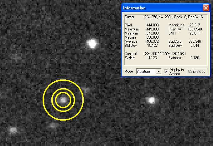
Figure 2. Flux measurement of an asteroid (15146) using
MaxIm DL. The photometry aperture circles are centered on the asteroid
and the real-time calculation of flux (referred to as "Intensity"by
MaxIm) gives a value of 1698 counts. The SNR of 29 allows for the
calculation of a SE on flux of 59 counts (1698 / 29). This image
is a median combine of 3 images, each an unfiltered 180-second exposure.
The time of this observation is used to determine that the air mass
for the asteroid was 1.32 (using TheSky). From Fig.1 we have:
(1) Cv = 21.30 - 2.5 * LOG ( Fc / g ) - 0.14 * m +
0.52 * C
We have values for the following observables: Fc = 1698 +/- 59, g =
180 [seconds], and m = 1.32. We don't know C, the
asteroid's
color. But knowing that its a main belt asteroid allows us to estimate
B-V = 0.86 +/- 0.40, which means that C = +0.20 +/- 0.23. Therefore,
(2) Cv = 21.30 - 2.5 * LOG ( 1698 / 180 ) - 0.14 *
1.32 +
0.52 * 0.20
Cv = 18.76 +/- 0.10
Notice that we've used an unfiltered image to estimate a V-band
magnitude. The uncertainty of 0.10 has two sources: SNR = 29 and C =
0.20 +/- 0.23. The SNR source is a "stochastic uncertainty" whereas the
asteroid color uncertainty is a systematic error. For the purposes of
creating a "rotation light curve" during one observing session only the
stochastic component needs to be used, so for that purpose Cv = 18.76
+/- 0.10.
Error Propogation for Above Example
I am a believer in the saying "A
measurement is useless without an uncertainty estimate." Notice
that I
used the word "estimate." This is because all but one of the
uncertainty sources are estimated calibration uncertainty; only the SNR
is measured, and it's a stochastic component. The example, above,
treated only one component of calibration uncertainty, the asteroid's
unknown color. In a later section I will show how to measure color
using the simplified magniutde equations, but for the balance of this
section I want to illustrate a more complete error propogation analysis
for the above asteroid example.
In the previous section I assumed that the constants and
coefficients in equation (1) are without error. These values are never
perfectly known. Their uncertainty leads to an uncertainty of the
derived magnitude. These uncertainties belong to a category called
"systematic calibration uncertainty." Here is a list of estimated
uncertainties for terms in equation (1) :
Zcv = 21.30 +/- 0.07
Kcv = 0.14 +/- 0.02
Scv = 0.52 +/- 0.10
Let's assume that the above uncertainties are uncorrelated with each
other, and propogate their errors. The following lists the SE
uncertainty for the asteroid brightness for all sources:
Zcv SE
+/-0.070 mag
Kcv SE
+/-0.026 mag
Scv SE
+/-0.016 mag
Cvr SE
+/-0.120
mag
SE from SNR +/-0.034 mag
Total SE (accuracy)= 0.146 mag accuracy)
Thus, we may conclude that the asteroid's V-band magnitude (based on
unfiltered observations) is Cv = 18.76 +/- 0.15 magnitude.
The saying "A measurement is useless without an uncertainty
estimate" uses the word "estimate" advisedly. This is because all but
one of the uncertainty sources are estimated calibration
uncertainty;
only the SNR is measured, and it's the principal stochastic component.
Estimating calibration uncertainty requires skill that can only be
acquired through experience. I've had about 4 decades of this
experience, but it shouldn't take a conscientious person that long to
do the above SE estimations.
There are other sources of systematic uncertainty, and I'll merely
list them here. I'll eventually create web pages that treat each of
them, and update this web page with links when they're available.
Flux correction when using small "signal
aperture" size (for improving SNR)
Interfering stars in the sky background annulus
Imperfect flat frames
Incorrect choice for x,y centroid location (serious
for faint objects)
For now, let's live life dangerously, and assume that these
additional systematic error sources are neglible.
Determining Color Using Iteration
In this section we're going to use V and B images to determine B and
V magnitudes that don't rely upon B-V assumptions. In other words, the
simplified magnitude equations can be used to determine B and V for any
unknown star. This can be done using a spreadsheet for iterating from a
starting B-V to a final, stable value.
Recall from Fig. 1 the following simplified magnitude equations for
B and V.
(3) B = Zb - 2.5 * LOG ( Fb / g ) - Kb * m + Sv *
Cbv
(4) V = Zv - 2.5 * LOG ( Fv / g )
- Kv * m + Sv *
Cbv
For the balance of this section I will
adopt values for the constants
and coefficients in these equations based on the calibration of my
telesope:
(5) B = 19.13 - 2.5 * LOG ( Fb /
g ) - 0.25 * m +
0.39 * C
(6) V = 19.56 - 2.5 * LOG ( Fv / g
) - 0.17 * m -
0.09 * C
where you will recall that F = star flux, g = exposure
time [seconds], m = air mass, and C (star color) is defined to
be
0.57 * (B-V)-0.30).
On the right side of the equation everything is either known or
measured, except star color, Cvr. When B and V images of the same star
exist we have information about Cvr, and the trick is to arrive at an
internally-consistent solution for B, V and Cvr.An iterative process
can
be used to determine these values. This is done
by first assuming that Cvr =0 (which is true for the typical star, for
which V-R ~ 0.30), then calculating a first iteration estimate for B
and V
(and therefore Cvr). After the initial iteration, producing B and V for
a
typical star Cvr
value, the new B and V values are used in a second iteration (using a
new Cvr = 0.57 * (B-V) - 0.30). Usually, only two or three
iterations are necessary to achieve a stable solution. Let's use a
specific example to illustrate the process.
Calibrating Telescope System
I will use observations from one night (2005.04.06 UT) to illustrate
the use of spreadsheets for determining the SME constants for each
filter.
Let's begin with how the observations were taken. MaxIm DL was used to
control an SBIG ST-8XE CCD, a Celestron CGE-1400 telescope, a SBIG
CFW-8 color filter wheel, and a Starizona MicroTouch wireless focuser.
TheSky 6.0 was used to display the location of Landolt areas, which
guided my selection of them for observing so as to produce a sampling
of air mass values for the night. Each Landolt area was observed with
filters B, V, R, I and C. A "sequence" of exposures was selected from
previously-created sequences that specified filter, exposure time and
number of exposures. A typical sequence consisted of 14 "lights" and 2
"darks." All exposure times were 10 seconds (unguided). The CCD cooler
was controlled at -24 C the entire night.
Image analysis involved the calibration of raw images using flats and
darks. The flats were taken at twilight (same observation night).
Several flats were made using each filter, and they were averaged to
produce a single flat for each filter. All flats had maximum counts
within the range 20,000 and 33,000 and exposure times within the range
1 to 20 seconds. All dark frames for the night (a few dozen) were
median combined to produce a single dark frame for use with all Landolt
images. After calibrating the Landolt raw images for a sequence, they
were median combined using auto-star alignment. This procedure produced
a single image corresponding to an observing sequence of a Landolt area
using a filter at one air mass value.
For example, Sequence #04 was made with a V-band filter of Landolt area
"LA1242" (i.e., RA = 12:42) at an air mass
value of 2.43 (as determined using TheSky), and it consisted of 12
useable images (only sharp images were used; I rejected those that
suffered from tracking errors or image wander due to mountain waves).
The next figure shows how star flux measurements of this #04 image was
used to determine SME constants using an Excel spreadsheet.
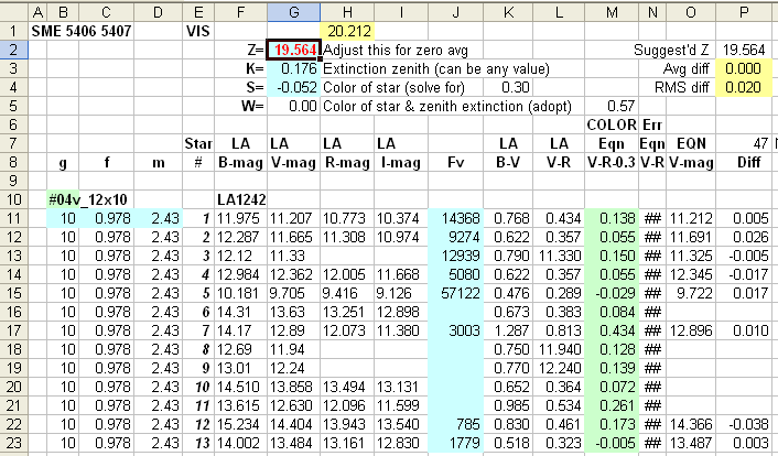
Figure 3. Part of an Excel spreadsheet showing observing
Sequence #04 information. The blue cells at the top are SME constants
(adjusted by the user), the blue cells on the left are exposure time,
aperture flux fraction (described below), and air mass. The blue cells
in
the middle are measured star fluxes. Landolt BVRI magnitudes are shown
(cells F11..I23). Columns "K" and
"L" show B-V and V-R star colors (based on Landolt valeus). Column "M"
is star color C = V-R-0.3
based on
an equation for converting B-V to V-R. Column "O" is SME magnitude
using the constants
in cells G2..G5). Column "P" shows the difference between the SME
V-magnitude and Landolt V-magnitude for stars 1 through 13. Cells with
no flux values correspond to stars that were too faint (SNR<70).
In this spreadsheet note the light blue cells. These require user input
or adjustment. The user must enter values for exposure time (B11),
aperture star flux ratio (C11) and air mass (D11). The user must also
enter star flux values in column J. The yellow cells provide feedback
for the adjustments (described in the next paragraph). The Landolt
magnitudes (F11..I23) can be copied from another sheet, so after they
have been entered into a spreadsheet once it should not be necessary to
enter them again.
The other cells are calculated. The message I want to convey here is
that once a spreadsheet has been created for using Landolt stars for
calibrating the telescope system, and once the user is familiar with
the spreadsheet, and, finally, once star fluxes have been measured and
entered into the spreadsheet, the work of solving for SME constants is
quite simple. The next paragraph explains this spreadsheet section in
more detail.
The zero shift constant, Z, is at cell G2. It should be
adjusted so that yellow cell P3 (average difference between SME
V-magnitude and Landolt V-magnitude) is zero. Cell P2 makes this
adjustment easy by suggesting the value that will accomplish this. For
a single image it is not necessary to adjust zenith extinction (cell
G3). When many stars are present the star color sensitivity
coefficient, S, in cell G4 can be adjusted for minimum "RMS
diff" in cell
P4 (RMS difference bewteen SME magnitudes and Landolt magnitudes). For
now we are not using W, the "air mass times star color"
coefficient (cell G5).
Column "C" contains the number 0.978. This is the ratio of star flux
using a small photometry aperture and a large one (9 pixel radius
versus 14 pixel radius, for example). I like using an aperture that is
as small as
possible in order to permit the use of a small sky background reference
annulus; this minimizes the chances of having interfering stars in
the background reference annulus. For faint target stars the use of a
small asperture increases SNR, which is another reason for having the
option of choosing a small signal aperture. SME photometry requires the
use of star fluxes that include the entire point-spread-function. The
compromise I employ is to choose a small aperture for measuring star
flux but correct these fluxes using a "flux response fraction" based on
the measurement of a bright star using both the small aperture and a
much larger one. This "flux response fraction," which I refer to by the
symbol "f" (as in cell C11), must be determined for each image. The
measured star fluxes (using the small aperture), shown in column "J",
are adjusted by dividing by "f" in the magnitude equation.
I recently switched from using star colors based on B-V to a version
based on V-R. All Landolt stars have B and V entries, but only ~1/4
have R
and I entries. As explained in the companion web page star color V-R is
correlated with B-V well
enough for use by SME photometry, an empirical linear equation can be
used to convert B-V to V-R with negligible error (usually). The
conversion is accomplished using V-R
= 0.01 + 0.57 * (B-V). After subtracting a typical V-R = 0.30 from
the converted V-R, I refer to this new star color as Cvr or
just plain C. In the figure they are shown in
column "M". Column "N" shows the difference between my converted
V-R-0.30 and Landolt's V-R-0.30, and the differences are small. (To see
a graph
showing Landolt V-R versus B-V, and the suitability of my conversion,
click V-R vs B-V ).
As images are added to the analysis the spreadsheet will grow downward.
As a convenience to the user graphs are also available for visualizing
a good choice for K and S that are uninfluenced by
outliers. This will be shown in the next figure.
At this point the reader should note that the above SME solution might
be adequate for use with another image at the same air mass for
converting a star's flux to a magnitude, provided we either knew or
were prepared to assume its color. The accuracy with which this could
be done appears to be 0.020 magntude, although this result is
based on only 8 standard stars. As will be seen when we add more
Landolt stars
to the analysis (next figure), the apparent SE accuracy that can be
achieved over a wide air mass and star color range is 0.017 magnitude.
The next figure shows a larger area of the above spreadsheet after a
total of 5 Landolt V-band images were included in the analysis.
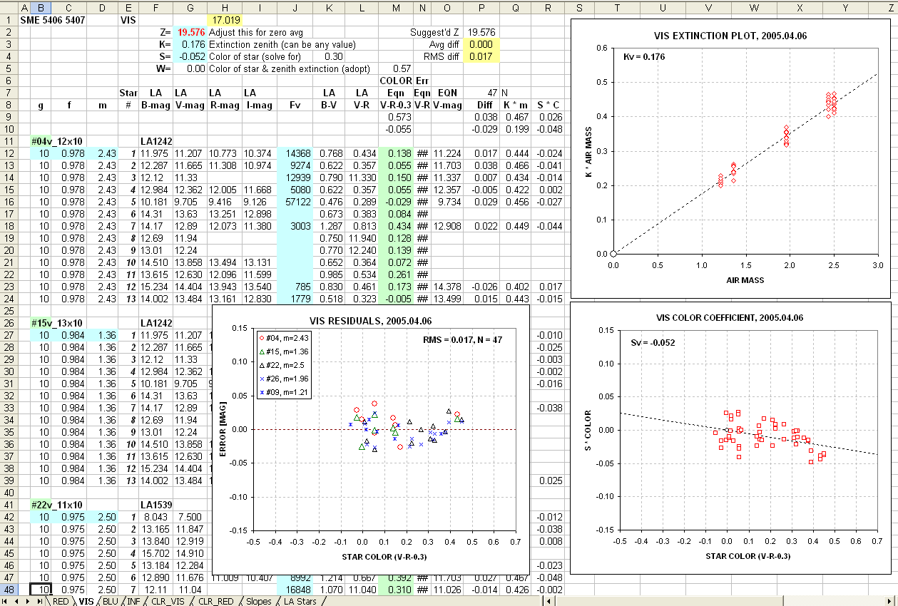
Figure 4. Screen shot of an Excel spreadsheet showing a
"solution" for V-band observations of Landolt star fields. Sheets like
this are present for each filter (see tabs at bottom). The two charts
on the right are used to determine zenith extinction and the star color
coefficient, as explained in the text. The lower-left chart shows
equation V-magnitude errors versus star color (V-R-0.3), from which it
was
determined that the RMS discrepancy with Landolt V-magnitudes = 0.017
magnitude based on 47 Landolt stars. Additional explanations are in the
text.
Let's analyze the additional material in this figure, one step at a
time. Some of this description will be a repeat of material presented
in the companion web page's "Calibrating a Telescope System."
Notice the new data for images #15 and #22 (others are present below
the screen shot boundary). A nice range of air mass values
is present, extending from 1.2 to 2.43. Note slightly different
aperture
response ratios, "f".
The chart in the upper-right shows a parameter "K
* air mass" versus "air mass." The slope of the fitted dashed line
corresponds to the zenith extinction coefficient for V-band, Kv.
The data is merely a plot of column Q versus column D, where column Q
is an equation for K*m (solved for using the SME for V):
(7) K*m = Z - V - 2.5 * LOG ( Fv / g ) +S * C
where C is the star color V-R-0.31 (derived from 0.57 * (B-V) - 0.30).
The fitted dashed line is specified by the zenith extinction value
specified by the user in cell G3.
If extinction had changed during the observing period it wouldn't
produce such a well-behaved (highly correlated) plot as seen here.
The lower-right chart is an analgous version used to determine the
color sensitivity parameter, S, where "S * C" is plotted versus C. The
slope of the fitted dashed line corresponds to the value for S, which
in this case is -0.07. The fitted line is determined by the value in
cell G4, and it must hinge through the origin, at 0,0. The lower-left
chart is a plot of SME V-magnitude minus Landolt V-magnitude, versus
star color. The RMS discrepancy with Landolt is 0.017 magnitude (based
on 47 Landolt stars), and
there is no residual dependence upon star color.
Similar spreadsheet analyses were performed for B, R and I, as well as
C
(clear filter). The next several panels of graphs are for B, V, R and I
filter data.
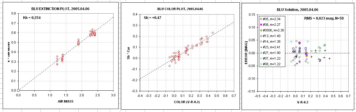
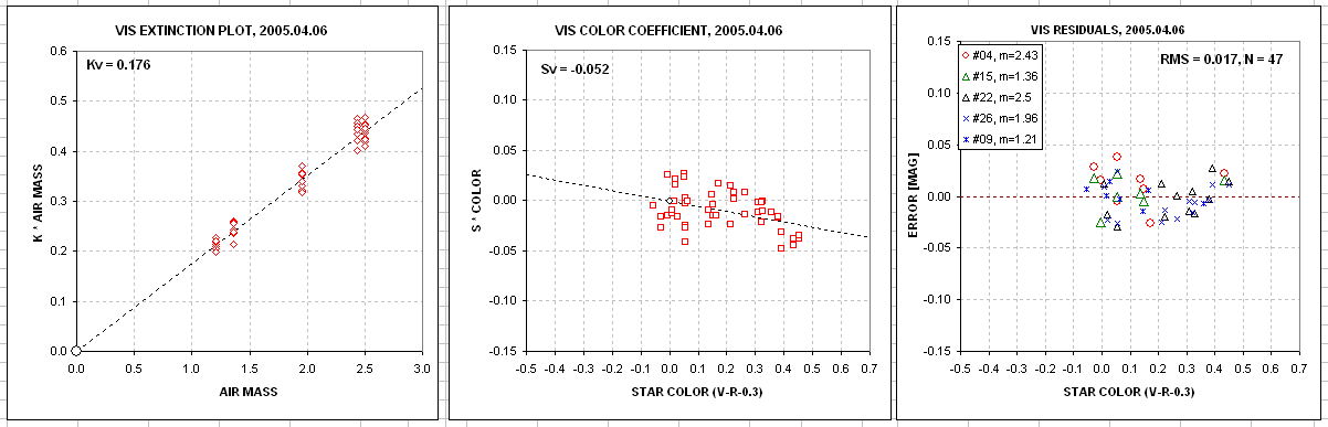
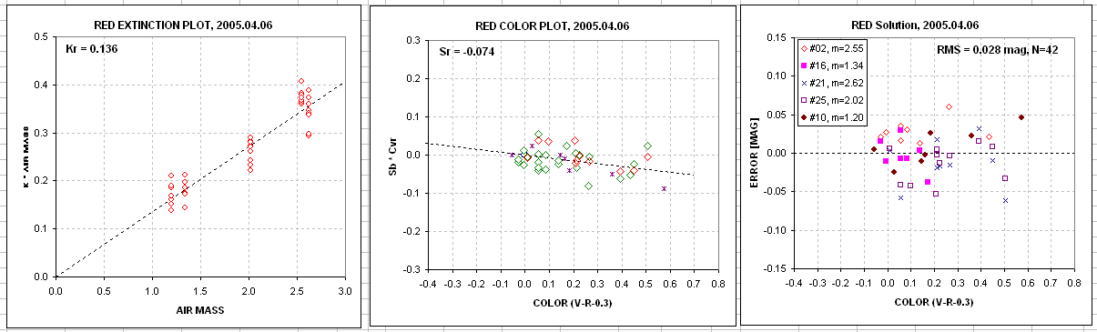
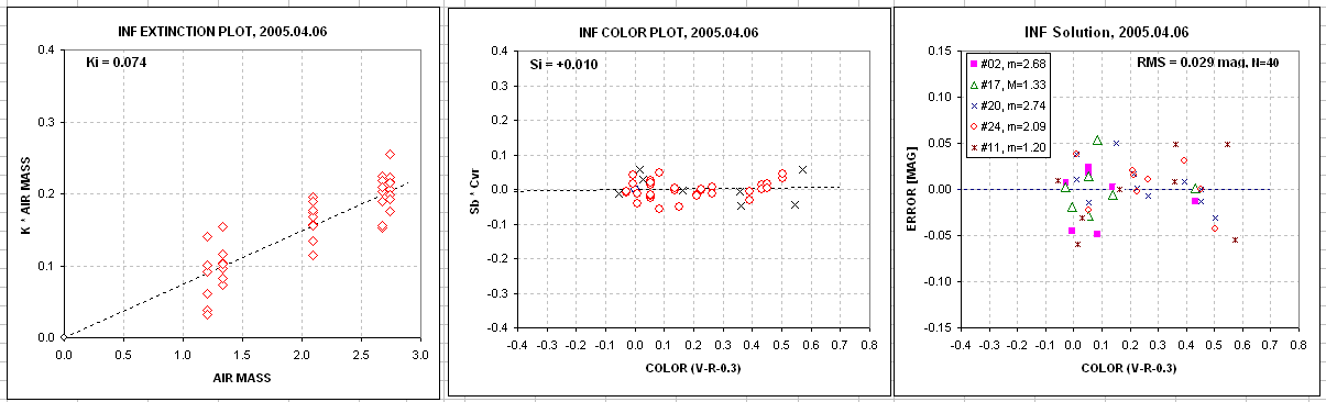
Figure 5. Screen shots of Excel spreadsheet showing a
graphs of parameters related to zenith extinction, star color
sensitivity, and residuals from truth (Landolt).
This set of graphs show a progression from high zenith extinction at
B-band to low extinction at I-band. Notice the different star color
dependencies.
The unfiltered fluxes were used to estimate V-magnitude and
R-magnitude, represented by the symbols Cv and Cr. The solutions
produced the following SME equations:
(8) Cv = 21.261 - 2.5 * LOG ( Fc /
g ) - 0.138 * m +
0.688 * C; RMS = 0.028, N = 35
(9) Cr = 20.940 - 2.5 * LOG ( Fc /
g ) - 0.138 * m -
0.025 * C; RMS = 0.025, N = 27
When the SME constant solutions for this observing date are combined
with results from 3 other observing dates the following equations are
been obtained:
Figure 6. Summary of SME constants derived from observations
of several Landolt areas on March 11, April 2, April 6 and April 9, 2005.
These equations use star
color parameter Cvr = 0.57 * (B-V) - 0.30, which is a close
approximation to V-R-0.30. The "air mass times star color term" was not
used for this analysis (W was set to zero).
The reason the "air mass times star color" term was omitted from
this analysis is that several dozen standard stars are needed to
distinguish bewteen the effects of that term from the preceding star
color term, and there weren't enough stars during this single night of
observations to solve for both W and S. The W
term can't be too important, because the RMS performance was good for a
wide range of star colors and air mass values.
Based on the RMS performances for the SME solutions for this observing
session it is fair to say that any stars in images taken during this
observing session could be asssigned BVRI magnitudes with an accuracy
of <0.03 magnitude, provided their star color was known. And if star
color wasn't known, it could be determined with an accuracy of ~0.05
magnitude using an iteration procedure described above and on the
companion web page. When C has an uncertainty of 0.05
magnitude, the
largest uncertainty this produces for a magnitude using the SME is for
B-band, and for that band the B-magnitude uncertainty attributable to
an uncertain C is 0.015 magnitude. TheV-magnitude uncertainty
attributable to a 0.05 magnitude uncertainty in C is 0.003
magnitude,
and for R-band and I-band the uncertainties are 0.09 and 0.00
magnitude. Therefore, the iteration procedure for establishing star
color is accurate enough to have negligible effect on the SME magnitude
determinations (based on this night's observations).

____________________________________________________________________
This site opened: March 25,
2005. Last Update: April
14,
2005