ARTIFICIAL STAR PHOTOMETRY
FOR GENERATING EXOPLANET LIGHT CURVES
Bruce L. Gary, Hereford Arizona Observatory
Introduction
The procedure described on this web page for creating light curves
using an artificial star will be referred to as Artificial Star
Photometry, or ASP. It has several advantages over other procedures,
such as the commonly used differential photometry: 1) extinction is
measured, allowing for the objective rejection of data influenced by
clouds, 2) image measurement is performed just once, even when the
identity of the variable star whose light curve is desired is
uncertain, and 3) several candidates for use as reference stars can be
evaluated for
variability (either real or induced by star field movement when the
flat field is not perfect) and the best combination can be specified
for ensemble photometry use in a spreadsheet. I will illustrate ASP
using real data of a suspected exoplanet system that turned out to be a
false alarm caused by a nearby eclipsing binary.
Image Measurement Phase
When a "comparison star" is used to measure the brightness
variations of a "target" star the image measuring program compares
"flux" values for the two stars. (Note: I'll use the term "comparison
star" instead of "reference star" when just one star is used as a
reference.) The flux of a star located within a signal aperture is simply the sum
of counts across a circular pattern of pixels minus the sum of counts
that would be expected if all signal aperture counts were the same as
the average within a sky background reference annulus. In MaxIm DL the
term "intensity" is used in place of flux. When the fluxes for a
variable and reference star "i" have been measured, referred to here as FluxV and FluxRi,
the magnitude difference dMi = 2.5 * LOG10 (FluxV / FluxRi).
If the reference star's magnitude is known, MRi, the variable star's
magnitude is simply MVi = MRi + dMi. If other stars are within the
field of view (FOV) they too can be used to estimate MVi. Thus, MV =
average { MVi }. This procedure is called "ensemble photometry."
This way of performing ensemble photometry assumes several things:
1) all reference stars are unaffected by flux variations caused by star
field drift with respect to the CCD pixel field (which will not be true
if the drifts are large and the flat field is not perfect), 2) clouds
do not drift through the FOV, and 3) the reference stars are in fact
constant. Note that this last point is unlikely to be important when a
set of "comparison" stars have been produced by a qualified observer
who will have observed the star field on more than one date for the
purpose of identifying non-variables for use as comparison stars. However,
exoplanet observers are usually working with star fields that don't
have a set of comparison stars that have been certified as constant,
and this means that all nearby stars that are available for use as
reference could in fact be variable (as the present case study
illustrates).
Image Processing Phase
My favorite image processing program is the same one I use during
observing to control the telescope and CCD camera, MaxIm DL - hereafter
referred to as MDL. It's possible that other programs can do the same
things, but since I 'm not familiar with them it will be up to the
reader who uses them to achieve the same functional results that I'll
describe for MDL.
Suppose a night's observations of an object to be monitored consist of
several hundred images. Because my RAM is limited to 768 Mbyte I can
only load ~200 raw images at a time (beyond which the hard disk is used
as virtual RAM, and that really slows things down). After loading the
first batch of raw images to MDL's work area, and calibrating them
using a master dark and flat, I "align" them using MDL's "Auto - star
matching" option. That operation does x and y shifts, plus a rotation
(if necessary), to all images to achieve alignment with the first image
in the list. Next I run the artificial star plug-in which places an
artificial star in the upper-left corner of all images in the work
area. I use Ajai Sehgal's 64x64 plug-in designed for use with MDL,
available at the Diffraction Limited web site. Here's an example of the
artificial star in an image (ignore the photometry apertures for now):
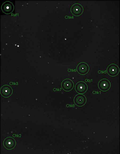
Figure 1. An image that has been modified by the artificial
star plug-in that placed a 64x64 "image" of a Gaussian artificial star
in the upper-left corner (labeled "Ref1"). Photometry aperture circles
have been placed at the target of interest "Obj1" and 8 other stars
"Chk1 ... Chk 8" that will be considered for use as reference stars
during the spreadsheet phase of analysis.
The artificial star consists of a Gaussian with FWHM = 3.77 pixels
and flux = 1,334,130 counts. After all images have this artificial star
applied I use MDL's photometry tool (invoked by the menu sequence
Analyze/Photometry). I select "New Object" mode and click on the target
of interest; it is labeled "Obj1" in the figure. The "Snap to centroid"
option is checked so it's not important to place the aperture circles
carefully on a star before left-clicking it. I next select the "New
Reference Star" mode and click the artificial star. It's not necessary
to enter a magnitude for it, even though I know that is is ~8.77 when I
use a R-filter, because that's a job for the spreadsheet. I next select
the "New Check Star" mode and click on a pre-assigned sequence of stars
that I decided earlier might be good reference stars (sufficient SNR).
In this case I included faint stars at the end of the sequence that
have poor SNR but might be the actual variable that was tentatively
identified with the brightest star within the survey telescope's
aperture circle. As we will see later, "Chk7" is an eclipsing binary
and "Obj1" was non-variable.
After all stars have been assigned their category in the image
presented to the user the same stars in all 200 other images have
automatically been identified by MDL. We are now ready to view a graph
of the magnitudes of all stars in all 200 images versus time. After
clicking "View Plot" we'll see a graph like the following:
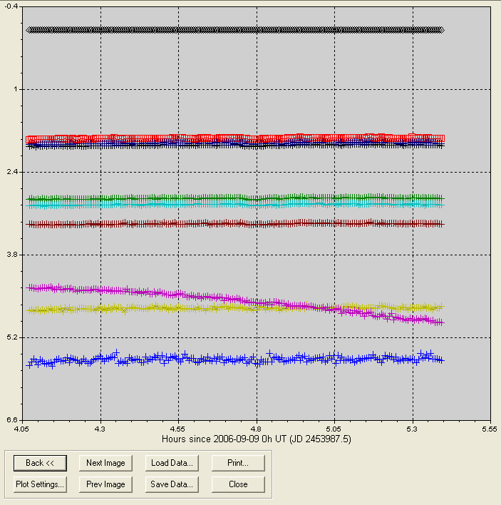
Figure 2. MDL's version of a light curve for the 10 stars
chosen for analysis (an object, a reference star and 8 check stars) for
200 images covering a 1.3-hour observing period. The single Reference
star was not assigned a magnitude, so it defaulted to zero, producing a
plot of gray diamonds at the zero level. One of the check stars shows a
fade. By clicking a plotted point for that star we can see that "chk7"
is highlighted on an image beside the graph.
Immediately upon viewing this graph it is apparent that one of the
stars is fading in brightness, and we know that it is the star labeled
"chk7" in the previous figure. Thus, we know that in the subsequent
analysis with a spreadsheet "chk7" is disqualified as a potential
reference star. We also know at this time that the target star, "obj1"
which is plotted by red squares in the above figure, appears constant -
at least within the limits of magnitude resolution for this plot. The
magnitude differences with respect to the reference star (the
artificial star) can be recorded as a CSV-file (comma separated
variables) by clicking on the "Save Data" button and giving this data
group a name, such as 1.CSV.
Processing the CSV-files
After all image groups have been processed by MDL in the manner just described we'll have several CSV-files
in a specific directory, named 1.CSV, 2.CSV, etc. At this point they
could be imported to an Excel spreadsheet for analysis, and that's what
most users will do if they try out ASP. For me it was more fun to write
a simple QuickBASIC program that reads all the CSV-files and calculates
many useful things that saves the spreadsheet from having to do it. I
compiled it as an EXE-file so in a fraction of a second this little
program converts CSV files to another text file (excel.csv) that has
many useful things calculated. The program reads an info.txt file that
includes the observer's site coordinates and the objects RA/Dec
coordinates (which can be edited by the user prior to use; as an option
all coordinate info can be altered by the program). The program
calculates LST from JD and site longitude. It calculates elevation
angle and hence air mass from LST, the object's RA/Dec and the site's
coordinates. It calculates the sum of fluxes for all "check" stars and
records this as a magnitude. This is used by the spreadsheet to
determine zenith extinction. Again, all of this can be calculated in a
spreadsheet and I expect that most users will prefer to do it that way.
Here's a screen capture of the first part of an excel.csv file:
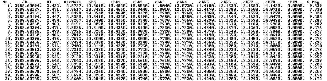
Figure 3. Sample output of program that reads CSV-files
(created by MDL) and records a file for import to an Excel spreadsheet.
The magnitudes given for all stars assumes a zero-shift constant that
has been established for my telescope system (for an R-filter) and it
is unimportant that it is likely to be in error by 0.1 or 0.2
magnitude. The file format can accomodate 9 check stars and when there
are only 8 the column for chk9 is all zeros. The last column, S-mag, is
the magnitude corresponding to adding the fluxes for all check stars
and is used in the spreadsheet for determining zenith extinction.
Spreadsheet Processing
I use an Excel spreadsheet with many pages. The first page is where the
text file (excel.txt, Fig. 3) is imported. It looks like this:
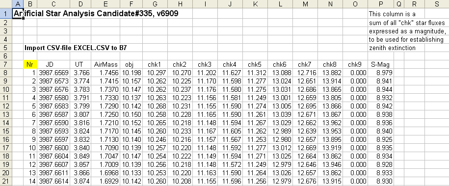
Figure 4. Excel spreadsheet with sample data imported to
first page. It has the same format as in the previous figure (the
numbers are different because the image groups are not the same).
The next page, below, uses data in the first page to determine zenith extinction.
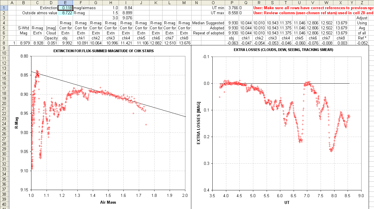
Figure 5. Spreadsheet 2nd page. The left plot is S-mag versus
air mass. It is "eyeball fitted" using a constant and slope in cells E1
and E2, corresponding to zenith extinction [mag/airmass] and a
zero-airmass intercept. The right plot is the difference between data
in the left plot and the eyeball fit, corresponding to an extra
component of loss not explainable by clear air extinction.
The zenith extinction value in cell E1 is 0.118 [mag/airmass],
which is a typical zenith extinction for my site for R-band. If the
skies are cloudless, there's no dew formation on the corrector plate,
and the tracking is good, the right plot would show no significant
departures from zero. In this case it had rained hard a few hours
earlier and the dew point was high, approaching ambient air temperature
(i.e., RH approaching 100%). During the observing session I
occasionally checked the flux of a certain star and when I noticed that
it was decreasing I turned on the dew heater. I had never used the dew
heater before so I changed settings until I thought I had one that was
working (at ~7.0 UT). The moon was full and several times I checked the
sky for clouds, and never saw any. I neglected to worry about this
problem until shut-down, when I saw with a flashlight that there was
light dew covering half of the corrector plate. Therefore, I attribute
the entire "extra losses" to dew on the corrector plate. As we shall
see this had no discenible effect on the results (unlike clouds, which
can have disastrous effects).
Columns E through M in this page are a prediction of what the star's
magnitude would have been if there were no clear sky extinction (i.e.,
a magnitude that would be observed outside the atmosphere, at zero
airmass, as predicted by the extintion fit). Cells Q4 to X4 are a median
of the good quality values in columns F to M. Columns Q through X in
this page are magnitude corrections that would be needed to correct a
particular star's brightness, for the image associated with that row,
to agree with the median value of all good quality entries for that
star (Q4 to X4). Since this magnitude correction takes into account
clear sky zenith extinction, the correction term can be large when an
image's "extra losses" is large. Presumably all stars in an image
affected by extra losses will be the same.
Column Z is where the user must make a judicious choice. It is an
average of some of the columns Q through X. Any star that is
"misbehaved" should be omitted from this average. This is where the
user is selecting reference stars. To evaluate the quality of a
reference star candidate refer to to the next figure, which is from the
next page in the spreadsheet.
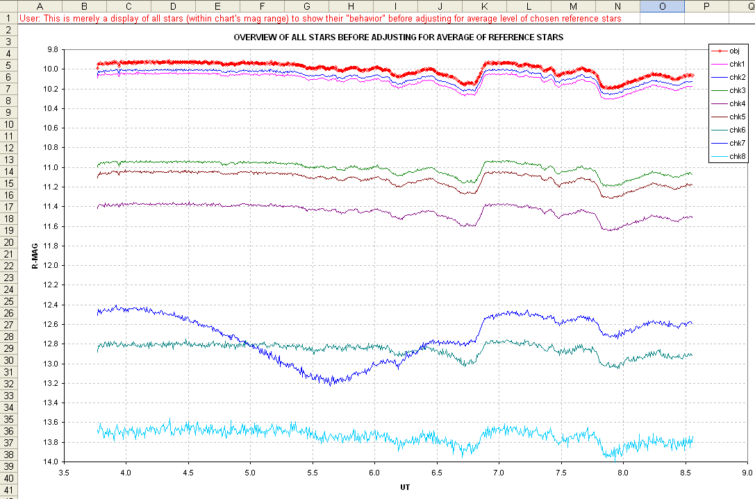
Figure 6. Extinction corrected magnitudes versus time.
This graph plots magnitudes that are corrected for clear sky extinction
but not corrected for "extra losses." If there were no "extra losses"
all traces would be featureless except for stochastic noise. They all
share the same "extra losses" features but the star "chk7" exhibits an
additional variation. This was expected based on the MDL plot of some
of the data (Fig. 2). We certainly don't want to include chk7 as a
reference star. The faintest star, chk8, has too much stochastic noise
to be useful, so it is also eliminated from consideration for use as a
reference star. I made the subjective decision of rejecting chk6 for
the same reason. My
tentative reference star selection is thus chk1, chk2, chk3, chk 4 and
chk5. This choise of reference stars is implemented on the previous
page by setting the equation for cells in column Z to be the average of
columns Q to U (it could just as well have been a median combine of
those cell values, which is safer when faint stars are used as
reference stars).
With this tentative choice for reference stars it is now possible to
correct for "extra losses" in creating a counterpart to Fig. 6.
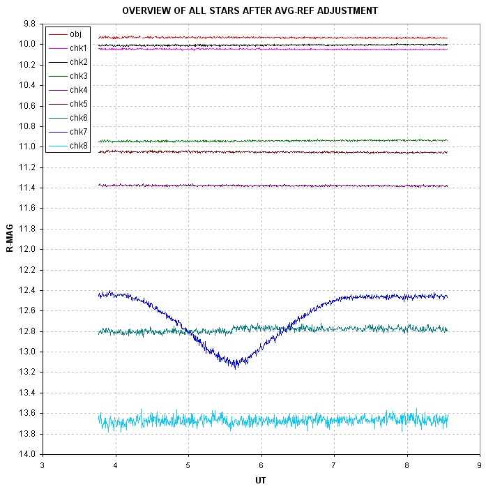
Figure 7. Same as previous figure except that the effect of "extra losses" have been removed by using 5 well-behaved reference stars.
Now we can see clearly that chk7 was transited by a companion star
during this obervation session. The transit depth is 0.66 magnitude,
which implies the existence of a transiting object far larger than any
planet. The reference stars, which are the 5 brightest chk stars, appear to be stable during the entire
observing period. This validates the reference star selection. This can
be seen a little better in an expanded scale accomodating only these
stars.
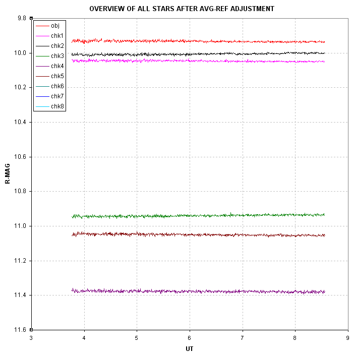
Figure 8. Same as previous figure except the magnitude scale
is expanded to show only the chosen reference stars (and the target
star, "obj1").
A slight drift exists for chk2 which is compensated by chk5. These two
stars are near the edges on opposite sides of the FOV. I try to avoid
using stars so close to the edge but in this case there were no other
bright ones near the target star. The result of having to choose edge
stars for reference is that some systematic effects can be expected in
the result of the target star's light curve, as is apparent in this
case in the next figure. It should be noted that for this set of 736
images the SBIG AO-7 tip/tilt image stabilizer kept the star field
fixed to the CCD pixel field with an RMS of ~1 pixel. Therefore, this
drift cannot be due to an imperfect flat field (unless the flat field
was changing with time, as might happen when dew forms on just one
side of the corrector plate).
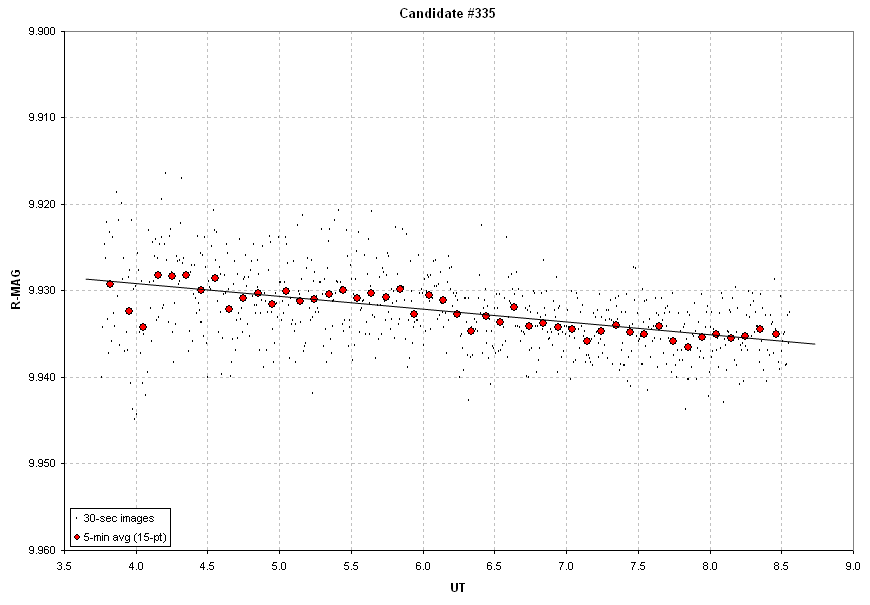
Figure 9. Target star's light curve for the 5-hour observing
period, during which there is a ~6 mmag drift . The 5-minute
non-overlapping averages depart from the sloped line with an RMS ~1
mmag.
It is apparent that no transit occurred for this star, and that was
the objective of the observing session. The target star's apparent
drift is surely an artifact of two reference stars drifing in opposite
directions by differing amounts.
Conclusions
It is important for the user to actually view the "behavior" of stars
before they are chosen to serve as reference stars. A spreadsheet is an
ideal tool for this because it allows the user to quickly see the
effect of changing the reference star selection. If a simple
differential photometry analysis is used, whether it uses one or
several "comp" stars, the user cannot see if any of those stars are
themselves variable. Nor can the user see the effects of poor SNR for
reference star candidates.
When it is necessary to establish which of several possible candidate
stars is varying (because the survey CCD had a large photometry
aperture) it is important to use an analysis procedure that does not
require repeated measurements of the images (because that's time-consuming). The ASP achieves
this goal by allowing all candidates to be included in the list of
stars to be photometrically measured (called "chk" throughout this web
page) while not commiting to the use of any of them as reference stars.
The merits of being as "close to the data" as possible are achieved
using the ASP. There are surely other ways to accomplish this, and if
the pst is any guide I will devise a procedure to supercede the ASP,
but whatever an observer does there is merit in being mindful of the
several pitfalls that traditional "comp" star analysis procedures may
remain hidden to the unwary user. This web page's "message" is to take
for granted as little as possible, and be vigilant in "looking for
trouble."
Related Links
XO-1 light curves
All-sky photometry
Photometry for Dummies
Bruce's Astrophotos (with many other links)
E-mail: b g a r y @ c i s - b r o a d b a n d . c o m
____________________________________________________________________
This site opened: September 11,
2006. Last Update: July 31,
2007