This web page describes the latest procedures used for fitting light curve (LC) submissions to the AXA.

Introduction

Amatuer LC data is almost always "noisier" than professional data. Often the level of noise does not permit a solution to be sought for some of the subtle aspects of LC shape. Starting April 14, 2008 I'll use a procedure that allows for these limitations without sacrificing the ability to extract mid-transit time from noisy data.

Another difference between amatuer and professional LC data is the size of systematic errors. There are two main systematics: 1) temporal trends (produced by polar axis mis-alignment that cause image rotation, which in turn produces trends as the star field moves across an imperfect flat field), and 2) "air mass curvature" (produced differences in star color between the target star and reference stars). The first effect is usually greater for amateurs because our polar axis alignment is rarely as good as to professional observastories, nor are our flat fields as good, usually. The second effect is usually greater for amateurs because our observing sites are at lower altitudes, where extinction is greater, and where the effect of star color differences is greater. Note that each star's extinction coefficient is slightly different depending on its color.

Because the two main systematic effects on LCs are greater for amateurs there's a greater need to address them and remove their effect when processing amateur data. In order for the AXA viewer to see how much systematics may be affecting the final LC I have decided to include two LC versions with each observer's data submission: 1) with systematics removed, and 2) without systematics removed.

Model Description

I use the term "model" reluctantly because my model is primitive compared with the models used by professionals. The following diagram illustrates what I'm calling a "model."

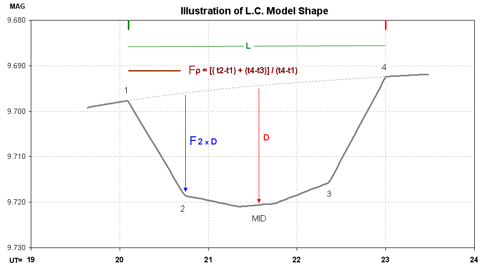
Figure 1. LC shape model used in fitting AXA submitted transit data. Trend and air mass curvature are present. First contact occurs at t1, etc. Descriptions are in the text.

This "model" includes 7 parameters (plust an offset), listed here:

    1) ingress time, t1
    2) egress time, t4
    3) depth at mid-transit, D [mmag]
    4) fraction of transit that's partial, Fp = [ (t2-t1) + (t4-t3) ] / (t4-t1)
    5) relative depth at contact 2, F2 (depth at contact 2 divided by depth at mid-transit),
    6) temporal trend [mmag/hour], and
    7) air mass curvature [mmag/airmass].

Mid-transit is "flattened" for a time interval given by (t3-t2)/4. Including an "air mass curvature" term requires that air mass versus time be represented by an equation including terms for powers of (t-to). I use a 4th power expansion with to set to the mid-point of the observations.

The interval t1 to t2 is "partial transit." Same for t3 to t4. The parameter "Fp" is the fraction of the total transit time that's partial. When a transit is "central" (impact parameter b = 0) Fp can be used to estimate the size of the transiting exoplanet (or brown dwarf star) compared with the size of the star being obscured.

The parameter "F2" is used to specify the amount of this limb darkening effect.

The interval t2 to t3 is not flat due to stellar "limb darkening."

Depth at mid-transit, D [mmag], can be used to estimate the size of the transiting exoplanet (or brown dwarf).

Least-Squares Fitting Procedure

Many steps are needed to perform a LS fitting of a model to data. Sorry for the detail in what follows, but some readers may want to know.

Deriving SE versus time

Every measurement has an associated uncertainty. If a region of data share the same SE (standard error) uncertainty, it is possible to deduce the value for SE by comparing a measured value with the average of its neighbors. This assumes that the thing being measured changes slowly compared with the time spanned by the neighbor values being averaged. Let's clarify this: the average of neighbors will be a good representation of the true value being measured provided the second derivative of the thing being measured is small (I won't belabor this since if you know about second derivatives you'll know what I'm getting at). I like using the 4 preceding neighbors and the 4 following neighbors, and I also prefer using their median instead of average (to be less affected by outliers). The median of 8 neighbors will itself have an uncertainty, but it will be much smaller than that for the measurement under consideration. Using the median of 8 neighbors leads to a SE on the 8 neighbors of ~ SEi ×1.15 × sqrt(1/7), where SEi is the SE per individual measurement (the 1.15 accounts for use of median instead of average). When a measurement is compared with this slightly uncertain version of "truth" the difference is slightly more uncertain than the measurement's actual SE. The histogram of many such differences will have a spread that is larger than SEi by 9%. My procedure for calculating SEi versus time during the observing session is to calculate the standard deviation of the "neighbor differences" data at each time step, then divide the entire sequence by 1.09.

This description left out one data quality checking step. The "neighbor differences" data can be used to identify outliers. When the absolute value of a measurement's neighbor difference exceeds a user-specified rejection criterion the measurement is rejected! Although the rejection criterion should depend on the total number of measurements, and should be set to a multiple of the SEi determined to exist at the timeof the measurement under question, I prefer to set the criterion to about 2.5 times the typical SEi for the observing session. This usually leads to a rejection of about 3% of the data (it would be 1.2% if only Gaussian noise were present). There's one other data quality checking step that is applied to some submitted data. When check stars (or even just one check star) are included in the submission it's possible to assess the amount of loss due to cirrus clouds, or dew on the corrector plate, or PSF spreading outsdie the aperture circle (due to seeing changes or focus drift), etc. I usually reject all data that has losses exceeding ~0.05 magnitude.

Solving for Model Parameter Values

Minimizing chi-square is a subset of least squares. Both assume that a measurement is actually a probability function having width given by SEi. The goal is to adjust model parameters to maximize the combined probability that the model "belongs" to the data. I suppose the word "belongs" should be explained.

For a single measurement with SEi specified there is just one parameter that can be adjusted for assessing "belong." The key concept is that every parameter value under consideration has a probability of "belonging" to the measurment, and this probability is simply the value of the Gaussian function at the parameter value's location. With two measured values the combined probability is the product of each probability. Since the Gaussian probability function is proportional to the inverse square of the difference, divided by SEi, the maximum combined probability will be achieved by a model that also minimizes the sum of squares of "model minus measurement divided by SEi." Chi-squared analysis involves finding a set of parameter values that minimize this sum, and it is equivalent to maximizing probability products. (Probability prodcuts is a Bayesian technique, and it lends itself to the case when probability functions are not Gaussian.)

There's one more feature available when minimizing chi-squared (or maximizing probability products). Outside information about likely values for model parameters can be explicitly made use of by treating them in a way similar to the way measurements are treated. If a model parameter has a known a priori probability function it can be included in the analysis. For example, if a Bayesian approach (product of probabilities) is used then whenever a model parameter is being evaluated the a priori probability that a value for it that is being considered can be included in the set of probability products (most of which come from comparing measurements with model predicted values). If it is assumed that all probability functions are Gaussian, then the chi-squared procedure can be used and the model parameter's difference from it's most likely value can be included in the sum of chi-squares. For each model parameter the additional term to include in the chi-square sum is "model parameter value minus most likely value divided by SE for the parameter." The effect of including this term is to reward model parameter values that agree with expectations, and punish model parameter values that stray too far from what is expected. For want of a better term I'll say that my auto-fit procedure minimizes "Super Chi-Squared" where:

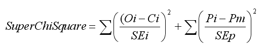
where measured magnitudes Oi and model computed magnitudes Ci are differenced and divided by measured magnitude SEi, then squared and summed for all measurements; followed by a set of model terms consisting of model parameter value Pi differenced with an a priori (most likely) value for the parameter Pm (based on a history of fitted light curves for the exoplanet in question) and divided by an a priori uncertainty of this parameter SEp, which are also squared.

Of course there is a potential danger in assigning a priori SE for model parameter values and punishing solutions that involve parameters that stray too far from what's expected. When an exoplanet transit has never been observed there is little information besides some basic physics for bounding parameter values (e.g., depth can't exceed 100% would be one example). There are occasions when using a priori SE for model parametsr is appropriate. Consider the following most common one for exoplanet transits. XO-1 has been observed on a few occasions with high precision, so the shape and depth and length of the LC is well established. For example, Fp = 0.26 ± 0.02, F2 = 0.83 ± 0.05, D = 23.8 ± 0.5 mmag (for R-band) and L = 2.91 ± 0.03 hours. Whenever a new high-precision complete transit observation is being fitted it is not necessary to makes use of this a priori information since the new LC data can be sued to solve for all parameters. However, when a low precision LC data set is to be fitted, or when only an ingress (or egress) was observed, it is not possible to solve for Fp and F2, and sometimes it is also not possible to solve for L or D with an expectation of reasonable results. Should this noisy or partial transit data set be rejected? No, if we constrain the parameters for whcih we have confidence and solve for the parameter(s) that may be changing, such as mid-transit time, we will be making legitimate use of prior knowledge as we try to learn about something for which we do not have prior knowledge. In the case of XO-1, for example, this permits us to make use of noisy LC data, or partial transit data, to solve for mid-transit time - a parameter that can be useful in a search for transit timing variations (TTV) produced by another exoplanet in a resonant orbit.

Professional LC data is usually very precise, for several reasons: large apertures have higher SNR and lower scintillation effects, professional observatories are at high altitude where extinction is less and image rotation is non-existent because polar axes are well aligned. Professional LCs therefore should have small temporal trends, small air mass curvatures and should never need to have model parameters constrained by a priori information. We poor amateurs, on the other hand, must work harder to overcome all the handicaps of not benefitting from the above list. This web page section is long because I need to explain the many procedure for overcoming amateur LC limitations.

I have decided to present two versions of every amateur LC so that the severity of sytematics and my success at removing them can be assessed. One LC version has systematics removed (which is what the professionals do) and immediately below it is another LC without the systematics removed. This dual presentation will be done for all submissions after April 15, 2008. I will use the first of these to illustrate what information is contained in the two LC versions.

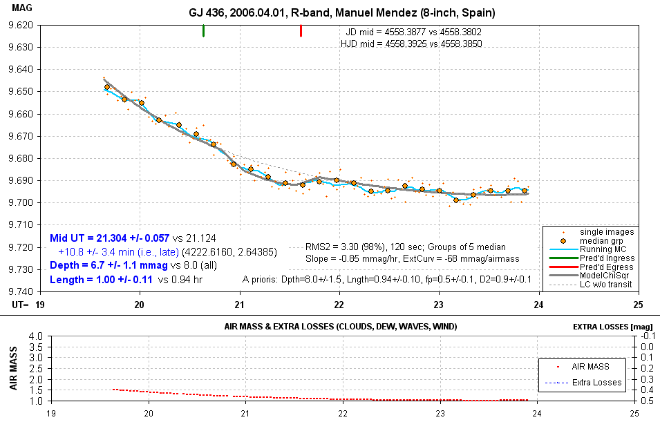
Amateur LC with a chi-square fit that includes a priori values for model parameters Fp, F2, D and L. Other details are described in the text. (fp is the same as Fp, f2 is the same as F2.)

Magnitudes from individual images are shown by small orange dots. Groups of 5 non-overlapping individual measurements ar shown with large orange symbols. A running average of the individual measurements is shown by a wavy light blue trace. The thick gray trace is a model fit. The gray dotted trace during the transit protion shows how the model would plot if the transit depth were zero.

GJ 436 is a very red star, and no reference stars are available that are equally red (and are bright enough for use as reference). Therefore it is common for LCs of this object to exhibit "air mass curvature" (since the target star and reference stars will have slightly different extinction coefficients). In addition to the air mass curvature this LC plot exhibits a temporal trend (usually due to imperfect polar axis alignment that produces image rotation). As noted near the lower-right corner the solved-for temporal trend coefficient (labeled "Slope") is -0.85 mmag/hour. The air mass curvature is also presented as -68 mmag/airmass (labeled "ExtCurv"). The same information group gives the single-image SE to be 3.30 mmag for a neighbor noise rejection criterion that leaves 98% of the data as accepted. The exposure time is 120 seconds. 

At the bottom central is a list of a priori model parameter assumptions. D = 8.0 ± 1.5 mmag, L = 0.94 ± 0.10, etc. My choice of SE for these parameters is twice their established SE from previous high-precision LCs.

The lower-left corner shows solved-for parameters whose solution was subject to the a priori constraints. The SE value for each parameter is obtained by adjusting the parameter value until chi-square increases by 2. Normally a chi-sqaure increase of 1 is required, but this assumes that either all parameters are "orthogonal" (do not mimic each others effects) or when a parameter is adjusted all other parameters are free to find their minimum chi-square solution. Since neither condition is met, I have adopted the custom, provisionally, of using a chi-square increase criterion of 2 instead of 1. The ingress and egree times call for a mid-transit time that is 10.8 ± 3.4 minutes later than the ephemeris used for predicting the transit. (It is known that the published ephemeris has a period that is too short, and LCs like this one are helping to establish a new period.)

The lower pael shows air mass. If reference stars had been included in the submission another curve would show "extra losses" due to cirrus clouds, etc.

Note that this LC was made using an 8-inch telescope. This is the smallest aperture used for observers who have submitted data to the AXA, and I salute Manuel Mendez for his successful observing.

The next figure shows the same data with the two systematics removed.

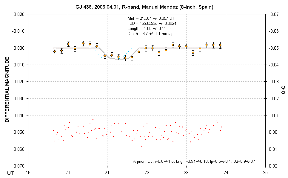
Systematics removed version of an amateur LC. Descritpion is given below. (fp is the same as Fp, f2 is the same as F2.)

The dashed blue trace is an offset LC shape showing when the transit was expected. The same grouping of 5 non-overlapping data are shown using the same orange symbols as in the previous plot. These data have SE bars that are based on the SEi versus UT (not shown) and divided by square-root of 4. The model fit is horizontal outsdie of transit, by definition. The small red crosses at the bottom  are residuals of the individual image measurements with respect to the model. The information groups are a repeat from the previous figure.

On the web pages devoted to each exoplanet I will present both graphs. Professionals probably don't publish the graph with systemtics present because their systematics are small and it is therefore not necessary to assess their importance. Amateur observations, however, should have the systematics illustrated so that anyone considering using the analysis results can be warned about errors that may remain after attempting to remove the systematics.

Plans for Future Automation

If you think this fitting procedure is labor intensive, you're right! I do it using a spreadsheet (LCx_template.xls, which you can download and use in the same way I use it). If Caltech's IPAC/NStED decides to include and AXA-like archive with my help, then I will work with Caltech to implement this procedure using a set of programs that chain to each other (a "pipeline"). Then the entire process will be painless, provided users have the discipline to submit their data in the required format (something only one of you has done for me). Wish me luck in getting Caltech to take over the AXA. It needs to be the responsibility of an institution, because I'm an old man!

If Caltech's NStED decides to not take over the AXA then I don't know what will happen to this site. In a parallel life I do work as a consultant for unrelated matters, so if anyone has an idea for funding me to automate the process I'll consider it.

TTV Strategy

When a well-observed exoplanet is under study for transit timing variations (TTV) there is no need to solve for Fp and F2, as this would just add to the uncertainty of the mid-transit time. It is also not necessary to allow length and depth be free parameters. Length and depth are usually well established but not with perfect accuracy. Therefore, for TTV studies I assign L and D their best estiamte SE, and assing Fp and F2 zero error, and proceed with the Super Chi-Square minimization procedure inspired by Bayesian Estimation Theory to solve for mid-transit time. SE on mid-transit time is evaluated by manually adjusting it so that Super Chi-Square increases by ~1.5, then finding a best set of parameter values for L and D (and the systematic parameters trend and AMC), and usually Super Chi-Square comes down to ~1.0. If it doesn't, then I adjust mid-transit time again, and solve for the other parameters. This process actually goes quite fast, and the resulting SE for mid-transit time is an objective evaluation that is valid if stochastic uncertainties dominate systematic errors.

One systematic that can't be dealt with using this procedure is a clock error that is not corrected before the observations, or at least measured afterwards and reported in the data submission file. So, please, observers, be diligent in monitoring your computer clock accuracy.

There will be an illustration of the TTV search in a couple months on the AXA for an exoplanet that appears to exhibit it.

Return to AXA home page.

This site opened:  April 15, 2008.  Last Update:  July 03, 2008