XO-1 EXOPLANET TRANSITS
Amateur Observations by Co-Author Bruce L. Gary
Hereford Arizona Observatory (G95)
This web page describes contributions to the
study of the XO-1 exoplanet system using observations with the Hereford
Arizona Observatory 14-inch amateur telescope during the past year (i.e., most of which precede the Space Telescope Science Institute press release on May
18, 2006). This web page has a Highlights section that summarizes "observational results"
for those not necessarily interested in the techniques used to achieve
them. Following that is a Detailed Descriptions appendix meant for amateurs interested in my observing and data analysis techniques. In the appendix I use the 2006.03.14 transit for a "how to" case study
tutorial, illustrating my belief that the two
most important considerations for achieving good exoplanet transit data
are: 1) keep the star field fixed to the same location on the CCD chip
for the entire observing session, and 2) use an R-filter. Since
I occasionally join with my neighbor (Dave Healy) in the use of his
32-inch RC I will also include those results on this web
page. The most recent update will always be at the top (the item and figure numbering are therefore in reverse order) .
HIGHLIGHTS
This section describes highlights based on
observations made at two observatories in Southern Arizona (Hereford
Arizona Observatory and Junk Bond Observatory). Items 1 and 3 were used
in the article
accepted for publication by the
Astrophysical Journal ("A Transiting Planet of a Sun-like Star" by McCullough
et al,
complete reference at bottom of this web page). Items 2, 4, 5 and 6
became available after the manuscript was submitted to the
ApJ
and are only available on this web page. Please understand that the
contents of this web page may be revised as I continue to figure out
how to process transit data. I'm just an amateur without the benefit of
internal review by colleagues. I welcome suggestions for improvement
and suspected errors.
Item 6) Combined R-Band Transit Observations
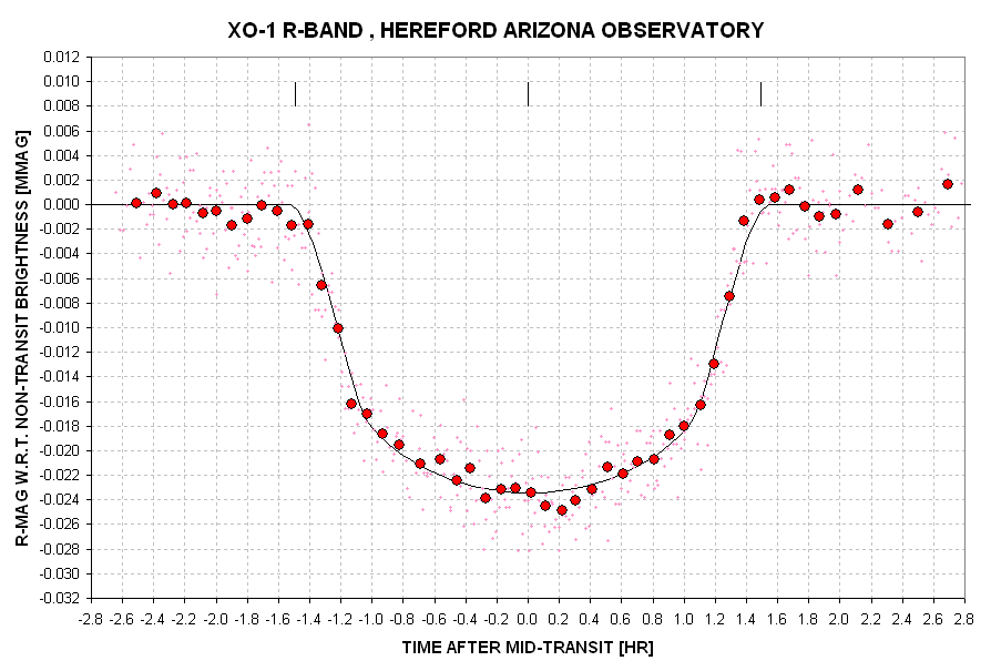 Figure 6. Combined 2006.03.14 and 2006.06.01 R-band light
curve. The pink dots are measurements of 1-minute exposures and the
filled red circles are 9-point averages (non-overlapping). The
mid-transit depth is 23.4 mmag and the duration is 2.8 hours (contact 1
to contact 4). The black trace is a fit using a very simple
transit model.The 9-point averages exhibit an RMS scatter with respect to the model of ~1 mmag.
[Hereford Arizona Observatory, 14-inch telescopes (Celestron CGE-1400
for 2006.03.14 and Meade RCX-400 for 2006.06.01), Hereford, AZ]
Figure 6. Combined 2006.03.14 and 2006.06.01 R-band light
curve. The pink dots are measurements of 1-minute exposures and the
filled red circles are 9-point averages (non-overlapping). The
mid-transit depth is 23.4 mmag and the duration is 2.8 hours (contact 1
to contact 4). The black trace is a fit using a very simple
transit model.The 9-point averages exhibit an RMS scatter with respect to the model of ~1 mmag.
[Hereford Arizona Observatory, 14-inch telescopes (Celestron CGE-1400
for 2006.03.14 and Meade RCX-400 for 2006.06.01), Hereford, AZ]
This figure is an average of two R-band transits (items 3 and 5, below)
using two different 14-inch telescopes at the Hereford Arizona
Observatory (MPC code G95). The data appear to "fit" a very simple
model, described at
model, which uses Rp/Rs = 0.144 (ratio of planet radius to star radius, both circular) and a linear limb darkening modeled using a
"1-cos(theta)" coefficient of 0.60.
Item 5) R-band Transit of June 1, 2006
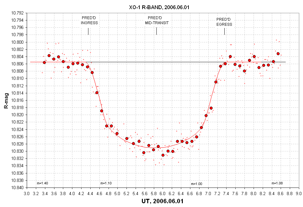
Figure 5. This R-band "light curve" is for the June 1, 2006
exoplanet transit of the 10.8 R-magnitude star XO-1 by the
Jupiter-sized planet XO-1b. The solid red circles are non-overlapping 5-point averages (spaced
6.9 minutes apart) of magnitudes from images with a 1-minute exposure time. An air mass trend correction of -0.004 magnitude
per air mass has been applied (maximum correction = 1.6 mmag), due possibly to color differences of the
reference stars and XO-1. The red trace is a model fit (described in the text)
shifted 1.6 minutes earlier than the predicted transit time. Mid-transit is at 5.829 ±
0.020 UT. The mid-transit depth is ~23.6 ± 1.0 mmag. (Measurements
precision suffered during this observing session due to several
episodes of downslope winds that caused star field movements that were
faster than my image stabilizer was able to follow.) [Meade RCX 14-inch telescope, SBIG AO-7 tip/tilt image stabilizer, SBIG
ST-8XE CCD; MaxIm DL for telescope/CCD/AO-7 control and image analysis; Hereford Arizona Observatory]
Mid-transit occurred 1.6 ± 1.2 minutes earlier than predicted (using Table 3 in the ApJ publication). This is consistent with the previous transit (4 days earlier) occurring 1.1 ± 0.5
minutes early. All mid-transit calculations are performed using HJD,
which are then converted to JD and UT. The timing of XO-1b transits
can be affected by another planet, especially if it is a resonant
orbit. Additional timings are needed to establish evidence for such a
planet based on timing departures.
Transit durations are worth monitoring in case there's any variation of
planet's orbit inclination or orbital velocity at the time of transit.
Instead of ingress to egress duration I choose to use something I'll
refer to as "1/3 depth duration" - the time between 1/3 of maximum
depth times. The 1/3 depth corresponds closely to the planet center
coinciding with the star's edge (for transit paths that come close to
the star's center (i.e., closer than ~3/4 of the star's radius; for
XO-1 the path comes as close as ~1/2 the star's radius). This "1/3
depth duration" geometry is convenient for calculating
the transit chord length and therefore orbit inclination. The three
dates have the following 1/3 depth durations: 2006.03.14 = 2.53
± 0.03 hours, 2006.05.24 = 2.56 ± 0.03 hours, 2006.06.01
= 2.56 ± 0.03 hours. So far there's no statistically significant
change in this measure of transit duration.
Transit depths at R-band are the same for the March
14 and June 1 transits, being 23.8 ± 0.5 and 23.6 ± 0.5 mmag, both of which are
less than the depth for B-band (next item)..
Item 4) B-band Transit of May 24, 2006
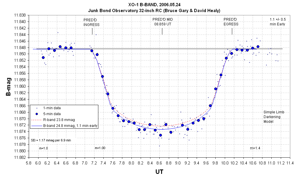
Figure 4. This B-band "light curve" is for the May 24, 2006
exoplanet transit of the 11.8 B-magnitude star XO-1 by the
Jupiter-sized planet XO-1b. Measurements of individual images (1-minute
exposures) are shown by small dots, and they exhibit a 1.96 mmag RMS scatter
(>6.2 UT). The solid blue circles are non-overlapping 5-point averages (spaced
6.9 minutes apart). The 5-point averages exhibit an RMS scatter of
1.17
mmag (non-transit portions >6.2 UT). An air mass trend correction of
+0.006 magnitude
per air mass has been applied (maximum correction = 2.4 mmag), due possibly to color differences of the
reference stars and XO-1. The blue trace is a model fit,
using a simple limb-darkening model, shifted 1.1 early with respect to the predicted transit time. Mid-transit is measured to be 8.640 ±
0.008 UT. The dashed red trace is from an R-band transit observation
(next item) made 2006 March 14 (with a 14-inch Celestron). The B-band mid-transit depth is ~24.8 ± 0.5 mmag (i.e., 2.31%), which is slightly larger than the R-band depth (23.8 ± 0.5 mmag) due to a steeper B-band limb darkening for the star XO-1.
(Data past 10.8 UT suffer from clouds.) [OGS Ritchey-Chritien 32-inch
telescope, David Healy (Director), MPC code 701, SBIG STL-6303E CCD
camera, MaxIm DL for CCD control and image analysis; Junk Bond Observatory, Sierra Vista, Arizona]
Limb darkening models for a sun-like star predict deeper transit depths
at B-band than R-band. This was shown by observations with the Lowell
Observatory Perkins 72-inch telescope (made by the Boston University
group led by Prof. Ken Janes, and reported in the ApJ article).
The present result is a confirmation of this color dependence, based on
observations made with two different (amateur) telescopes and a model
fit using Rp/Rs = 0.144 and simple linear limb darkening model with a
"1-cos(theta)" coefficient of 0.60. The May 24 transit occurred 1.1 ± 0.5
minutes earlier than predicted. A WWV radio check was made of the
computer clock which was the source for FITS header time tags, and the
computer clock was accurate to ~1 second.
Item 3) R-band Transit of March 14, 2006
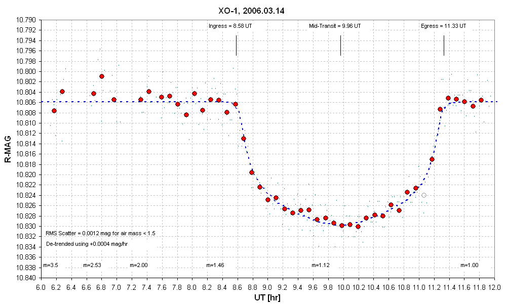
Figure 3. This "light curve" is for the March 14, 2006
exoplanet transit of the 10.8 R-magnitude star XO-1 by the
Jupiter-sized planet XO-1b. Measurements of individual images (1-minute
exposures) are shown by dots, and they exhibit a 2.6 mmag RMS scatter
(for air mass < 1.5). The red circles are non-overlapping 5-point averages
(spaced 6.5 minutes apart). The 6.5-minute averages exhibit an RMS scatter of 1.2
mmag (air mass < 1.5). A trend correction of +0.0004 magnitude
per hour has been applied, due possibly to color differences of the
reference stars and XO-1. The dashed blue trace is an empirical fit,
forced to be symmetric about mid-transit (9.96 UT). The open circle is
suspect data when a hair dryer was used to evaporate frost from the
telescope's corrector plate. The mid-transit depth is ~23.8 mmag (i.e., 2.2%).
[Celestron 14-inch telescope, SBIG AO-7 tip/tilt image stabilizer, SBIG
ST-8XE CCD; MaxIm DL for telescope/CCD/AO-7 control and image analysis; Hereford Arizona Observatory]
This light curve was made during an exceptionally calm and clear night
with better than usual "atmospheric seeing." The SBIG AO-7 tip/tilt
image stabilizer kept the star field fixed with respect to the CCD
pixel field (RMS ~1 pixel) which minimized degrading effects related to
an imperfect
"flat field" (a calibration to correct for "vignetting"). Although
slightly better quality observations of this star
have been obtained in April, at times when no transits were scheduled
to
occur (with a Meade RCX-400 14-inch
telescope), this is my most successful observation of an
exoplanet transit to date. Following this "Highlights" section I
present a tutorial illustrating observing and
analysis procedures that I recommend for exoplanet transits. Dr. Peter
McCullough used this transit, plus observations of several
others by myself and other team members beginning in June, 2005, to
establish an
orbital period for XO-1b of 3.941534 +/- 0.000027 day.
Item 2) Search for Additional Planets
During April and early May there were no transits
of XO-1b that could
be observed from my longitude. I used this non-transiting interval to
search for transits by other planets in the XO-1 system and to
determine if the star XO-1 exhibited brightness variations when no
transit was in progress. A
total of 37.5 hours on 20 nights have been used in this search. The two
transit features that would be produced by another planet, and which
could be detected using my amateur equipment for a planet as small as
1/3rd the
diameter of XO-1b (1/9th the transit depth, or 2.6 mmag) are: 1)
ingress or
egress changes in brightness during the observing session, and 2)
night-to-night differences in
brightness caused by an observing session being brief and confined to
between ingress and egress.
A search of each night's observing session showed no
ingress or
egress features. Also, the night-to-night average
brightness did not change in a way that could be interpreted as
produced by a transit exceeding 5 mmag, which represents this study's
null result for additional planet transits. The constancy of XO-1
appears to be better than 5 mmag during the 4-week observing period.
The following graph shows nightly R-magnitude averages for XO-1 and a
nearby faint check star.
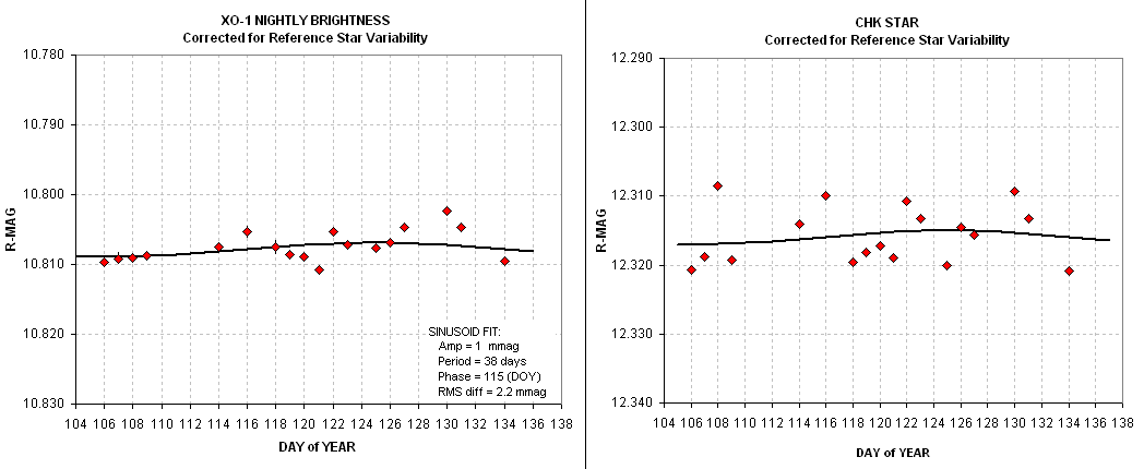
Figure 2. Nightly brightness of XO-1 (when XO-1b is not
transiting) and a nearby check star (1/4th as bright as XO-1).
Observing sessions were typically 2 hours long. A correction
has been applied for small variations of reference star brightness.
Error bars are stochastic SE and do not include
unknown systematic effects that apparently exist at the 3 mmag level.
The sinusoidal "fit" to the XO-1 data (repeated in the check star plot)
has an amplitude of 1 mmag and a period of 38 days, but data
uncertainties are insufficient to claim that the variation is real.
[Meade RCX400 14-inch
telescope; Hereford Arizona Observatory]
XO-1's brightness appears to have been stable
during the 4-week observing period. This result is somewhat dependent
upon my analysis of reference star variations and the removal of their
effect upon XO-1 brightness. A detailed description of this analysis is
given at
ReferenceStarVariability.
I want to mention that this is my first observing
project with a newly-purchased Meade RCX400 14-inch telescope. This
telescope, mounted on an
equatorial wedge, is ideal for exoplanet monitoring for the following
reasons: 1) it's a fork mount (no meridian flips to interrupt
observing), 2) the tube is made from low thermal expansion material (no
focusing changes
that would interrupt observing), 3) collimation is easy (no excuses for
coma effects on photometry), 4) sturdy mount and OTA (same polar
alignment every night, less shaking due to wind), 5) good tracking
(easier to keep the star field fixed with respect to the CCD pixels),
and 6) the RCX optics produce good image quality for a larger FOV,
which means a larger CCD chip can be used, which means there's a
greater likelihood of including bright reference stars in the FOV,
and this translates to smaller Poisson and scintillation components of
uncertainty for the
exoplanet's ensemble photometric brightness measurement.
If the Jupiter-sized planet XO-1b has a moon the planet and moon will
orbit around their center of mass (i.e., their "barycenter"). It takes
23 minutes for XO-1b to cross the star's edge (contact 1 to contact 2).
If, for examle, XO-1b has a moon with mass 1/10 that of XO-1b in an
orbit that's just as large as Io's orbit around Jupiter (scaled up by
1.3 so it has the same ratio to its planet's radius as Io's orbit has
to Jupiter's radius), then every 2.7 days XO-1b would orbit around the
barycenter with a total movement of ~60% of its diameter. This would
produce transit timing shifts with an amplitude of ~7 minutes (~14
minutes peak-to-peak). Given that transit timings are the same as
predicted to within ~2 minutes, such a large moon can be ruled out.
However, we cannot yet rule out a moon in the same orbit with a mass
1/70th that of XO-1b. Amateurs should be able to achieve timing
accuracies of ~1/2 minute per transit. This means there's an
opportunity for asmateurs to constrain the mass of any hypothetical
XO-1b moon to the level ~1/300 the mass of XO-1b (or some combination
of orbital distance and mass). Since the Hubble Space Telescope has
apparently eliminated the possibility of a moon for exoplanet HD209458b
(from the shape of the transit) it is a "long-shot" project to be
looking for effects of a moon orbiting XO-1b.
Item 1) Creation of Photometric Sequence
There are two reasons to establish a photometric sequence of the XO-1
star field. First, the brightness of star XO-1 is used to derive a
distance, which in turn is used to determine a most probable stellar
mass and radius, and at a later stage this is needed to solve for the
planet's mass and radius (and density). Second, in order for different
observers to compare observations made at different times it is useful
to adopt magnitudes for nearby stars so that they may serve as a common "reference."
I
observed standard star fields established by Landolt (1992) on two
dates (2006.02.25 and 2006.03.14) for the purpose of establishing a
B, V, Rc and Ic photometric sequence for stars near XO-1. The Landolt
regions
were near the celestial equator at RA 04:52 and 12:42, and there
were 28 stars bright enough for the establishment of constants for my
telescope's "zero shift" and "star color sensitivity." The observations
were
timed so that air masses were the same for the Landolt stars and XO-1,
and they
were taken close in time in order to reduce any
effects of temporal extinction changes. Additional information about
these all-sky observations can be found at
AllSkyXO1.
Eight
potential reference stars were chosen for this analysis. The two sets
of Rc magnitudes were in good agreement (average difference = 0.005
magnitude). Here's a finder chart for the 8 stars.
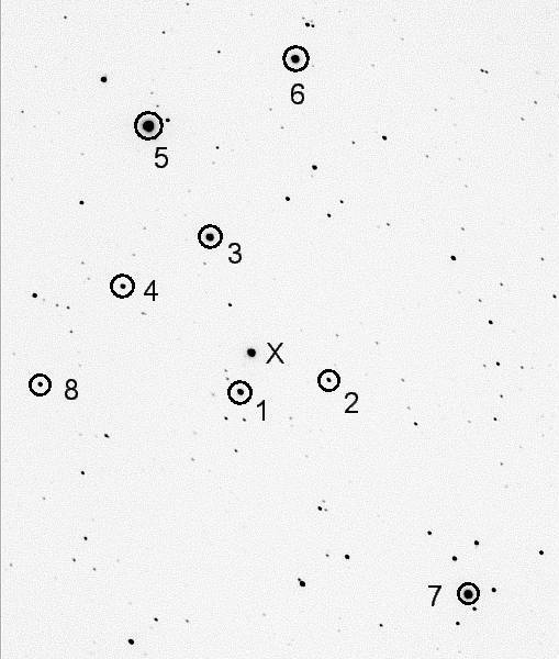
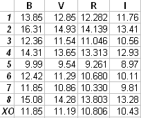
Figures 1a. Eight stars for which all-sky BVRcIc magnitudes have been performed. An "X" is next to XO-1. FOV = 16 x 21 'arc. Figure 1b. Table of all-sky magnitude determinations.
The estimated SE accuracy for these stars is:
B SE = 0.04 magnitude
V SE = 0.03 "
Rc SE = 0.020 "
Ic SE = 0.03 "
_______________________________ This is the end of the HIGHLIGHTS section ______________________
APPENDIX: DETAILED DESCRIPTIONS
Links Internal to this Web Page
Introduction
Site and Hardware
Software for Telescope Control and Analysis
Planning a Typical Night's Observations
Exposure Times
Observing and Reduction Logs
Flat Frames
Dark Frames
Focusing
Automating Observing Sequence
Image Stabilization and Tracking
Maintaining an Observing Log
Image and Data Analysis
Spreadsheet Analysis
Updated Finder Chart
Final Photometric Sequence
Searching for Other Planets in the XO-1 System
Poisson Noise & Scintillation Noise (compared with observed precision)
Transit Ingress & Egress Schedule for May and June, 2006
Related Links (other XO-1 transit observations, transits of other exoplanet systems, etc.)
References
Introduction
The star XO-1 is located in the constellation Corona Borealis, at RA =
16:02:11.6, Dec = +28:10:11 (see
CB for a zoom sequence showing XO-1's location). I have measured its brightness (all-sky
photometry) to be B = 11.85, V = 11.19, Rc = 11.806 and Ic = 10.43. The
exoplanet XO-1b has an orbit that causes it to transit in front of the
star every 3.941534 days (McCullough et al, in press). The star is very
similar to our sun in size, mass and surface temperature. This new
solar system is ~200 parsecs away (650 light yeaers). The planet has a
mass ~0.9 times that of Jupiter, and its spherical-equivalent size
is ~1.3 times that of Jupiter (McCullough et al, in press). The planet's
density is ~0.57 times that of water, which is slightly less than the
density of Saturn (0.69 times water) and much less than the density of
Jupiter (1.33 times water). As described in the article by McCullough
et al, the exoplanet system was discovered in early 2005 by a
wide-field survey (McCullough et al, 2005). Four amateur observers contributed
to the confirmation of the transit light curve shape being planet-like
starting in mid-2005: Tony Vanmunster, Ron Bissinger, Paul J. Howell
and Bruce L. Gary. Dr. Peter McCullough confirmed the planet
identification using Doppler velosity observations in early 2006. So
far no transits have been found beside those produced by XO-1b.
This rest of this web page emphasizes one night's observations with
a
14-inch telescope. Links are included that treat related issues, such
as subsequent searches for additional planets in the XO-1 system, other
transit observations by this observer (in 2005 and 2006), other
people's web sites, and my all-sky observations used to derive a BVRcIc
photometric sequence for stars near XO-1. Much of the following
material is "tutorial" in nature, as it is meant to illustrate the way this amateur conducts exoplanet observations.
Site and Hardware
The "Hereford Arizona Observatory" (HAO) is used for observing gamma-ray bursts,
supernovae light curves, cataclysmic varible super-hump monitoring, and faint
asteroid rotation light curves. The observatory has a Minor Planet Center
designation of G95. HAO is located in the rural community of
Hereford, in Southern Arizona, 90 miles southeast of Tuscon, 7 miles
from the border with Mexico. The altitude and coordinates are 4660
feet, -110.2377, +31.4522. A mountain range is located 5 miles west of
the site, reaching an altitude of 9400 feet, which too frequently produces downslope winds that degrade "atmospheric seeing."
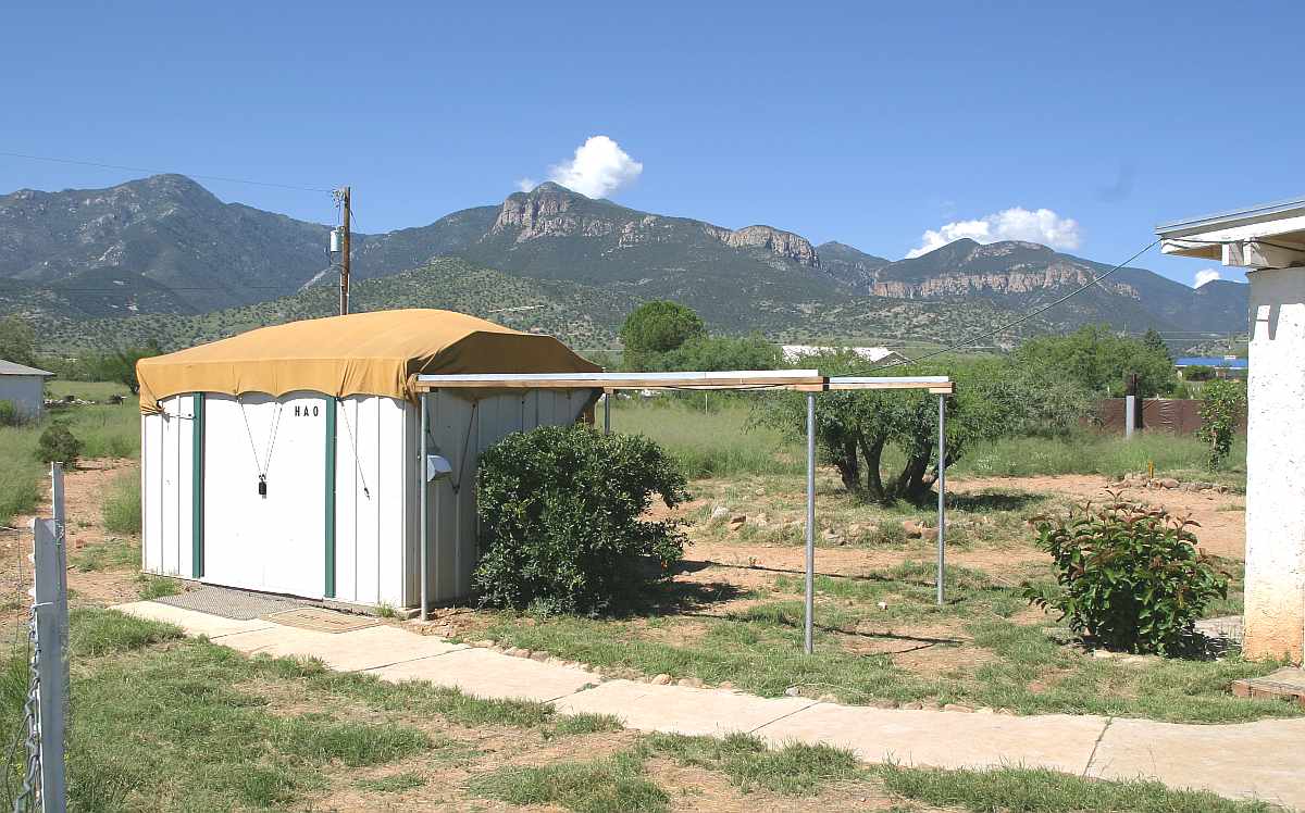
Figure A1. View of HAO, looking southwest. The two mountain
peaks are at 9400 feet, or 4700 feet higher than the HAO. Downslope
winds occur almost every night (at ~1-hour intervals), and they may
originate in the canyon between the two peaks (as radiatively cooled
air becomes dense and starts falling through ambient air and spreads
out over the valley).
The telescope used for the 2006.03.14 transit observation is a 14-inch aperture Celestron Schmidt-Cassegrain,
model
CGE-1400. The GE means "German Eqauatorial," which means trouble! Every
meridian crossing requires a manual "meridian flip," plus associated
changes to software settings for image orientation and tracking
directions. I'll never buy a GE again! The telescope is located in a
"sliding roof observatory" 70 feet from my house office "control room."
Cables are buried in conduit for control of the telescope. I focus
using a MicroTouch/Feathertouch focuser (made by Starizona); it's a wireless focuser that
adjusts the primary mirror. A wireless video camera and microphone are
used to monitor observatory conditions from the remote office control
room. (Since these observations were made I sold the Celestron and have
bought a Meade RCX400 14-inch fork-mounted telescope; no more meridian
flips for me!)
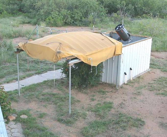
Figure A2. The canvas-covered roof is open showing the
Celestron 14-inch telescope. Note the two buried conduits entering the
building; one is for AC and the other is for several control cables.
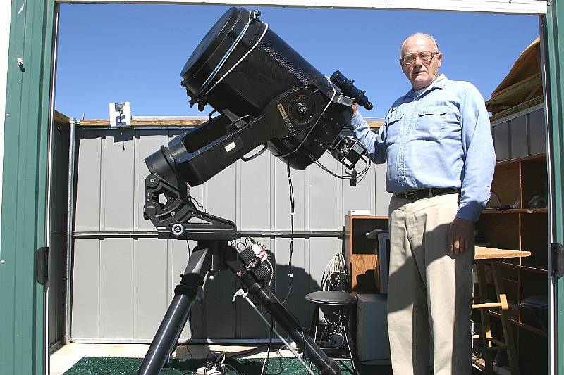
Figure A3. My new Meade RCX400 14-inch telescope. (This is a great telescope for exoplanet observing, as I describe at paean.)
The CCD is a SBIG ST-8XE, with 9-micron pixels, 1530x1020, and a
"237" autoguider chip next to the main chip. The filter wheel is a SBIG
5-position CFW-8. The CCD and CFW are mounted at the Cassegrain
location behind a focal reducer lens and image stabilizer. The image
stabilizer is a SBIG AO-7, which works with the autoguider chip's image
to produce tip/tilt adjustments at ~3 Hz. The focal reducer is located
~4 inches from the CCD chip, which quadruples the FOV solid angle and
affords smooth flat fields. (If the focal reducer lens is too close the
flat fields have too much structure that's different for each filter.)
The image scale for this configuration is 0.97 "arc/pixel. The FOV is
24.7 x 16.5 'arc. For this particular exoplanet transit project the CCD
assembly is rotated so that the longer FOV dimension is north-south,
with a bright star in the autoguider's FOV.
My computer clock uses AtomicTime, a utility that updates the
computer clock every 3 hours. I verified that it was correct by noting
that it agreed with a wireless (WWV signal) clock to within 1 second.
I have a Davis "wireless" weather station near the
observatory with sensors at 11 feet AGL. It transmits signals to a
receiver in my office where a data logger records many weather
parameters; these data are available for download to a dedicated weather
computer. The weather computer produces a graphical
display of wind speed and direction, temperature, dew point and RH, and
barometric pressure. The wind and temperature traces can be used to
predict "atmospheric seeing" degradations (~5 minutes ahead of time)
since the
downslope winds begin with a slow rise of wind followed 5 minutes later
by a rise of temperature (due to adiabatic heating as the air that is
sinking out of a nearby canyon).
Software for Telescope/CCD/focuser Control and Analysis
I use MaxIm DL for control of telescope pointing, CCD camera and
AO-7 image stabilizer. MaxIm DL uses MaxPoint, also from Diffraction
Limited, to correct for polar alignment errors and mount flexure; this
assures accurate pointing (but does not improve tracking). MaxIm DL has
two ways to accomplish aperture photometry. The on-the-fly display of
star flux at the cursor location is a crude tool since it does not
reject comic ray defects or interfering stars in the sky background
annulus. If used with care it is a very useful tool however (I use it
for all my all-sky photometric sequence analyses). The second way to
perform aperture photometry is with MaxIm's photometry tool
(Analyze/Photometry). A set of images (~30) can be processed using ensemble
differential photometry, and this is what I use for analyzing exoplanet transits.
The photometry tool creates CSV-files that can be imported into a
spreadsheet. More on this later.
TheSky 6 is a "planetarium" program that shows the sky's star field.
It is an indispensable tool for planning an observing session and in
reducing data. In the afternoon before a night's observing I use TheSky
to schedule what to observe and when. For all-sky photometric sequence
observing it is important to schedule observations of Landolt star
fields at the same air mass as the region of interest (ROI). TheSky
shows when the ROI transits, which requires a 10-minute break in
observing to accomodate a manual meridian flip and software settings
changes. For data reduction it is convenient to use TheSky to determine
air mass for image groups.
Finally, I like spreadsheets. I now use Excel, inspite of it's
orientation to business users. I have template spreadsheets that
facilitate the kind of analyses that I frequently perform.
Planning 2006.03.14 Observations
For the night of March 13 (2006.03.14 UT) I used TheSky to
schedule all-sky observations of two Landolt star fields before XO-1 transit. I did this partly to verify that the candidate
reference stars near XO-1 had not varied from the date that I
first established their brightnesses (2006.02.25). TheSky showed that XO-1 transited at 11:59 UT (4:59 AM). This was
~45 minutes past egress, and also just before dawn, so I decided to
terminate observations at transit. The scheduled ingress, at 08:47 UT
(01:47 AM), occurred while XO-1 was rising through an elevation angle (EL)
of 49 degrees. XO-1 was scheduled to rise through EL = 15 degrees at 11:00
AM, so I scheduled observations 15 minutes earlier of the Landolt star
field LA1242 (located at RA = 12:42 near Dec = 0). XO-1 would be at
LA1242's elevation (~40 degrees) 2 hours later. Shortly after sunset on
this night I scheduled observations of LA0452 using V and R filters
(for another project). The two R-band observations of Landolt stars
would provide a check that extinction was not changing.
I prefer R-band for exoplanet work for several reasons:
Extinction is low for R-band (typically 0.11 mag/air mass at my site), the CCD's
QE is high and the observed flux for a typical star is greatest for
R-band (being 36% of clear), and scintillation is lower than for B or V due to R-band's longer
wavelength. Unfiltered observing is unwise because reference
stars with different colors fade differently with air mass (due to extinction); this could cause an exoplanet to
have trends that are difficult to remove (especially when pre-ingress
and post-egress times are not observed).
Exposure Times
Exposures must be kept short enough that the
brightest reference
star is not saturated. For this star field the brightest
star has R-mag = 9.28 which requires that my exposures be no longer
than 60 seconds. If "atmospheric seeing" gets too good the telescope
has to be purposely de-focused in order to assure that no pixels are
saturating.
As an aside, for large apertures very short exposure
times are required. This has two penalties: 1) image download times can
be comparable with exposure times (leading to low duty cycles), and 2)
scintillation increses as exposure times are shortened. For example, a
32-inch
telescope would require 11 second exposures instead of a 14-inch
telescope's 60 seconds (assuming both CCDs used 16-bit A/D converters).
If the download time per image is 8 seconds the duty cycle for the two
telescopes would be 88% and 58%. Poisson noise per image will be the
same, since for each telescope the maximum counts for the brightest
star will be ~30,000 counts, but the larger telescope acquires more
images per unit of observing time (3.1 images per minute for the
32-inch versus 0.9 images per minute for the 14-inch). Scintillation
depends on both aperture and exposure time, and smaller apertures are
net winners on this consideration (see the section on scintillation,
below). The large aperture penalty for this example is 32%, but the
3.5-fold greater number of images per observing minute is more
important. The point of this aside is to show that although larger
apertures are better for exoplanet observing their advantages are not
as dramatic as for faint object observing.
Another consideration is when to start observing the
exoplanet. I
decided to start when it was low in the sky in order to have sufficient
air mass range to search for air mass related systematic errors. My
range extends from air mass, m = 3.5 to 1.00. Experience shows that
good data is usually not possible until air mass is less than 1.5 or
2.0.
Observing and Reduction Logs
I'm a firm believer in maintaining logs for all
observing sessions.
At the top I record my goals and plans for the night, as well as sky
conditions (cloud cover and type, plus wind). The plan includes what to
do and at what times. For decades I would use only ink for the
observing log, and
pencil for the reduction log, but since retirement I've relaxed that
"rule" and I now use pencil for both with a rigorous rule of not
altering my observing log (except as carefully noted). For me, an
observing log is more sacred than the bible!
I noted in the March 14 observing log that the weather was excellent. The sky was cloudless and the wind was
calm, conditions that I categorize as "photometric."
Flat Frames
After opening the observatory I turned everything on, placed a
T-shirt over the telescope aperture (secured by a bungee cord), and
manually pointed to zenith. I set the CCD cooler to 0 C (a modest
cooling seems to improve my flats; after the flats I specify a colder setting for use with the ROI). Flat frames were taken
for each filter to be used that night (plus Clear, in case an
interesting GRB was announced while observing). Exposure times
ranged from 1 to 20 seconds. Shorter than 1 second might produce
an artificial vignetting from the way the CCD shutter operates.
Exposure times were carefully changed to assure that the maximum count
was in the range 28,000 to 34,000. This is about half the maximum for a
16-bit A/D converter, and for my CCD model this assures that saturation
effects are minimal. I specified that dark frames be taken with the
flats as a precaution for hot and dead pixels.
I took 11 flats with the R-filter (plus others with the V- and
C-filters). I used to "median combine" the flats for each filter, using
"normalize," but I've discovered that the normalize feature does funny
things to image intensity scaling that produces subtle defects in the
final flat frame. Image averaging is a safer procedure, provided each
individual image to be averaged is first visually inspected for cosmic
ray defects. I averaged the R-band flats in 3 groups and compared,
noting that slight changes had occurred as the exposure times
increased. I weight-averaged the flats to produce a master flat for the
night, giving preference to the longest exposure set. The R-band master
flat had a vignetting pattern that was smooth except for one persistent
dust donut, and at the corners the response was ~65%. I try to not use
reference stars in the corners even though I believe that the flat
frames correct vignetting to the 1% level.
Dark Frames
I believe in establishing a master dark frame for each temperature
and exposure time setting to be used for the ROI. The first half of the
night's observing session was with a CCD cooler temperature of -15 C,
while the XO-1 observations were at -25 C. I took a set of 40 dark frames
at -15 C (60-second exposures) during a dinner break, and later a set
of 16 dark frames at -25 C (before the XO-1 observations). I don't deal
with bias frames since I always use dark frame exposure times that are
the same as my ROI exposures. (I don't like the variable results of
correcting for CCD temperature and exposure when calibrating with dark
frames made under different conditions). By creating a master dark
frame from 16 individual dark frames, median combined, the master dark
frame has a pixel noise that is about 1/3 of the individual ROI pixel
noise. After subtracting such a master dark frame from a ROI light
frame the pixel noise increases by only 11%.
Focusing
My Celestron tube shrinks with cooling temperature, so focusing has
to be monitored. I always focus unfiltered, and add previously
established offsets for each filter. Past midnight the focus doesn't
change much, so I usually monitor it by noting star "shapes." My
collimation is such that a defocused star changes shape to an oval with
an orientation that I can "read" for the direction of needed focus
change. Between exposures I change the focus by a small amount and note
the effect on star shape. This procedure allows me to continue
observing without an interruption of the automatic expsoure schedule.
At the beginning of the observing session my best focus gave FWHM = 4.2
"arc. This was established from a plot of the best of several FWHM at a
sequence of focus settings. Not great seeing, but acceptable for
photometry. I made several adjustments (as described above) throughout
the night, and 60-second exposures had typical FHWM that ranged from
3.5 to 4.4 "arc.
There may be occasions when it will be desireable to intentionally
maintain a defocused condition. For example, saturation of the
brightest pixel must be avoided, so in order to accommodate a very
bright star for use as a reference star a defocused image can be used
to lower the brightest pixel value to below saturation (~50% of
full-scale for non-ABG CCDs). The star's total flux will be unaffected,
and the star's Poisson noise won't be affected. The only penalties are
1) signal aperture noise will be higher (due to having to use a larger
radius), and 2) interfereing stars may be present in the sky background
reference annulus (due to having to use a larger reference annulus).
The appendix provides conceptual tools for assessing the penalty for
using a larger signal aperture.
Automated Exposure Sequence
MaxIm DL has an automated exposure sequence feature that allows the
user to specify a filter, exposure time, binning, delay time after each
exposure, repeat count for the sequence, file name for each exposure
and destination directory for recording images. I chose R-filter, 60
seconds for each exposure, binning of 1x1, and a 10-second delay after
each exposure (as explained in the next section). Each sequence consisted of 10
exposures, numbered 0 thorugh 9, and I set the sequence repeat count to
99.
Image Stabilization and Tracking
In the abstract I stated that it's important to keep the star field
fixed to the same location on the chip for the entire observing
session. Doing this reduces the effect of flat field imperfections. In
fact, if you are successful in keeping the star field fixed it should
not be necessary to even employ flat field corrections (provided FWHM >> 1 pixel). On this date I
succeeded in keeping the stars fixed to within a few pixels for the
entire 5-hour main exoplanet observing session. Here's how I
accomplished it.
My AO-7 image stabilizer adjusts the tip/tilt mirror at ~3 Hz to keep
the guide star's image fixed, thus keeping the star field on the main
chip fixed. However, my polar axis was ~0.2 degrees off, so there was
a drift that typically caused the AO-7 to reach it's tracking limit in
~4
minutes. MaxIm DL is supposed to "nudge" the telescope drive in the
required direction whenever the AO-7 exceeds a user-specified
correction threshold. However, since a lightning strike near my site
last summer I have been unable to use that feature. So, I have
intentionally specified a 10-second delay after each exposure for
manually nudging the telescope in a way that should be done
automatically. (Hey, I knew I was getting a new scope a month later, so
it wasn't worth fixing!) This makes for a lot of extra work! It meant
that I had
to stay close to the control computer to perform the nudges, which I
usually perform after each exposure. Since my exposure time was 60
seconds I had to "attend" to nudging every minute - which I did for
the entire 6-hour XO-1 observing session!
If the polar axis is adjusted to be close to perfect, it's true that
fewer manual nudgings would be required but another problem would
exist. Whenever a Declination nudge in the opposite direction is needed
there would be a backlash issue. For my scope the backlash is now ~15
seconds of nudge, and this would make Dec reversing difficult. (Yes, I
could tighten the Dec backlash gear again, but that would mean another
polar alignment session, MaxPoint calibration - and hey, I'm getting a
new scope in a amonth!)
Maintaining the Observing Log
I'm wary of the degrading effects of cirrus clouds, dew or frost
accumulation on the telescope corrector plate, the need for focusing
changes, wind-driven smearing, waves in the atmosphere that cause
smearing along one direction and other unforseen problems, so I perform
a minimal
processing of each raw image as it is downloaded.
Here's a sample of my observing log for 2006.03.14.
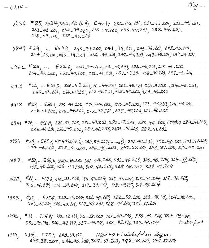 Figure A4. Sample observing log (page 3 of 4). Left columns
is UT start time for a sequence. Next number for each group is the
observing sequence number, then elevation. Then there are 10 coded
number groups, one for each image, describing FWHM and 3
digits for the kilo-counts flux of Reference Star #5 (Fig. 5a). Focus adjustments are also
noted.
Figure A4. Sample observing log (page 3 of 4). Left columns
is UT start time for a sequence. Next number for each group is the
observing sequence number, then elevation. Then there are 10 coded
number groups, one for each image, describing FWHM and 3
digits for the kilo-counts flux of Reference Star #5 (Fig. 5a). Focus adjustments are also
noted.
At the bottom of this observing log page, at the end of the observing
sequence #33, that started at UT 10:46, there's a notation "Must be
frost." The next observing sequence has the notation "Finished hair
dryer." At that time the outside air temperature (at roof level) was 28 F, the dew
point was 19 F (RH = 70%), and I was concerned about frost forming on
the corrector plate. What aroused my concern? Let's take a moment to
describe what I record for each opbserving sequence.
Look at the sequence that starts at 10:46 UT (sequence #33). It starts
out with "..." that refers to the info at the top of the page: object
is X634 (part of an earlier name for XO-1), RED filter, and AO-7 set to
0.4 second exposure times. Then it
states that elevation angle was 74.8 degrees (at the start of the
sequence - serving as a reality check when using TheSky later to derive
air mass). Then there's a set of coded numbers, one for each image. The
first one is for image 330. The notation is "330_42.199." This means
that X634 had a FWHM of 4.2 "arc (actually smaller since my aperture
was set to maximum radius), and the star's flux started out 199
(actually it was 199,033). I keep track of the need for focusing with
the FWHM entry, and the possibility of cirrus clouds and dew or frost
with the star flux. The set of star fluxes for this sequence is: 199,
200, 200, 200, 200, 198, 197, 198, 196, and 194. The downward trend at
the end alerted me to the need to check the sky or frost on the
corrector plate. So I went outside, the sky looked clear (thanks to a
full moon for showing cirrus), so I concluded there was frost on the
corrector plate. I checked it with a flashlight, and used a hair dryer
to blow warm air on some frost that had formed on the corrector
plate (while pointed at zenith and taking data for Sequence #34). As
noted for the last sequence on this page I finished the hair dryer
treatment at ~11:05:40 UT, with the possibility of ruining images 341 -
344 (with a hair dryer obstructing some of the aperture and a
flashlight checking for frost). The post-hair dryer star fluxes did
indeed rise, ~4%, showing that the frost had indeed been accumulating
since maybe 10:36 UT (using the other star flux notations to establish
the beginning of the downward trend).
Did the hair dryer episode affect exoplanet observations? If we're
trying for 1 or 2 mmag precision then surely placing a hair dryer over
the aperture and shining a flashlight should have had some effect! OK,
yes, it dropped the exoplnet observed brightness by 4mmag! This can be
seen in Fig. 1, where there's a low point at 11.07 UT.
This example of frost effects illustrates the value of paying attention
in real-time to downloaded images and quality checking to avoid
unrecoverable problems. If I hadn't noticed the decrease in star flux
due to frost I might have lost the entire egress.
Image and Data Analysis
After a nap and breakfast, there remains a short session of dealing with images and a longer session of spreadsheet analysis.
A group of ~30 images are loaded into MaxIm DL. They are subjected to a
"Calibrate All" command which applies a dark frame subtraction and flat
frame division. Next I use the MaxIm DL Photometry tool to batch
process the group of 30 images using ensemble differential photometry.
For XO-1 I used 5 reference stars that surrounded XO-1 (I now use only
4 reference stars; the 12.30 star is too faint, and adds noise to the
XO-1 result).
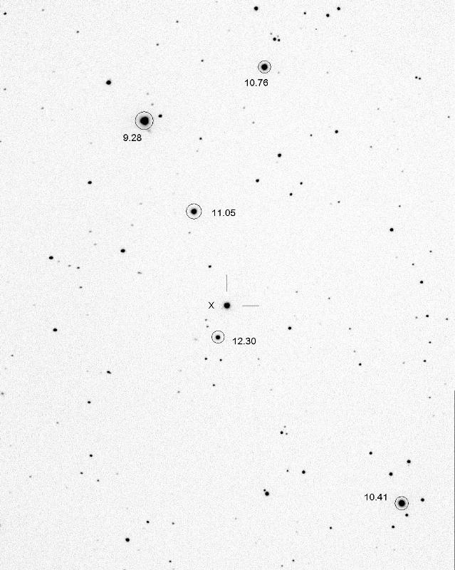 Figure A5. Finder chart showing my 5 reference stars
(ensemble photometry) and a
set of R-magnitudes. These aren't the actual R-mags but they're close
to
the apparent R-mags I get using my telescope without correcting for
star color. FOV = 16.4 x 20.6 'arc (cropped version of an original).
[Note: starting in April I have omitted use of the star labelled 12.30
since it added noise to the XO-1 observations.]
Figure A5. Finder chart showing my 5 reference stars
(ensemble photometry) and a
set of R-magnitudes. These aren't the actual R-mags but they're close
to
the apparent R-mags I get using my telescope without correcting for
star color. FOV = 16.4 x 20.6 'arc (cropped version of an original).
[Note: starting in April I have omitted use of the star labelled 12.30
since it added noise to the XO-1 observations.]
The reference star south of XO-1 is fainter than XO-1 by a factor of 4 (R-mag = 12.3 vs 10.8) but I
used it as a reference star (mistakenly, I now believe) because of its
close proximity to XO-1. Three stars are brighter, and
with ensemble the average magnitude for all of them is used to
establish the target's magnitude. That 12.3 magnitude star has a SNR
~250 for my 60-second exposures, so it's magnitude is uncertain by ~4
mmag based on CCD noise stochastic arguments. Scintillation is probably
comparable, and is experienced by all stars in the FOV. The ensemble
differential photometry result for XO-1 is uncertain by 2.6 mmag per
60-second image (based on a spreadsheet analysis of this transit).
Averaging the results from 5 images leads to a stochastic uncertainty
for the exoplanet of 1.2 mmag per 6.5-minute group of 5 average,
plotted as red circles in Fig. 1.
Before performing the ensemble differential photometry it's important
to select a signal aperture radius that includes most of the flux from
stars for the range of seeing conditions of the observing session. In
changing signal aperture radius there's a trade-off of SNR and "flux
recovery ratio," which I'll call
Fr (where
Fr is the ratio of flux for a given aperture radius,
r, to that for a large radius). Theoretically, going from very small radii to large, SNR increases, reaching a maximum at
r = 0.75 * FWHM (assuming a Gaussian PSF), then begins to decrease to low values for large radii. At the same time the plot of
Fr grows monotonically from zero to one. The "sweet spot" is a radius such that
Fr ~99% (which is my subjective estimate). As seeing varies
Fr will vary, but it should vary the same for all stars in a specific image (assuming minimal coma), so the fact that
Fr
is as low as 99% does not imply that there will be 1% uncertainties in
the resultant magnitude estimate (this would be true for all-sky
analyses, however). The relevant parameter is the change of
Fr
with location on the image, and my crude estimate of this (for my
present collimation setting) is that setting r = 12 pixels when FWHM =
4 pixels, leads to
Fr values that are the same (~0.99) for all
reference star locations, with a max-to-min variation of 0.0018 (RMS =
0.0007). Therefore, errors from this source are likely to be 0.7 mmag
for typical images.
MaxIm DL's photometry tool "asks for" reference star magnitudes, and it is
not
important to use accurate values. Even if one of the reference stars is
a long period variable and has a brightness different from the assumed
one by possibly a magnitude, little harm is done to the ensemble
photomtry result for the target. For example, according to my
spreadsheet analysis the above 5 reference stars differed from their
assumed magnitudes (based on observations of 2006.03.06) with an RMS =
0.035 mag. Their average difference was 0.00 mag. I conclude that none
of the 5 reference stars are variable on timescales of a few days. The persistent differences for
the 5 reference stars (of one night with respect to another) is
probably related to differences in the flat field used for the two
observing dates. But it really doesn't matter that each refernce star
could be wrong by as much as 0.038 mag since the star field on the CCD
chip did not move more than a few pixels for the entire observing
session.
After MaxIm DL performs its ensemble differential photometry, assigns
the unknown target star a magnitude, and calculates the image's
mid-exposure time in JD units, the user may then record the results
as a CSV-file (comma separated values). These CSV files can then be
imported to a spreadsheet.
Spreadsheet Analysis
Each CSV-file import has a title header line that can be removed by
deleting its row. Thus, after all CSV-files have been imported there
are no row gaps between data. The data should be uniformly spaced in
time since an observing sequence with a large repeat count there were
no pauses between sequences. For my observations all image mid-exposure
times in the spreadsheet are 78 seconds apart.
Occasionally a cosmic ray artifact will be present near the center of a
star image. If this occurs for a reference star (or the target star)
the ensemble photometry result will be affected. Therefore, outlier
target star data must be identified and rejected. My favorite routine
for this is to calculate in a spreadsheet column the difference between
a target magnitude and the average of the 4 nearest neighbors. Visual
inspection of this column readily shows where bad data exist. I found
only one such outlier among the total image count of 224 images
(excluding the first 0.6 hour, which corresponds to air mass greater
than 2.5).
Once outliers have been deleted I calculate group-of-5 averages. Each
group is for different data compared to the neighboring group average
(i.e., it's not a sliding boxcar, which can be misleading). The
group-of-5 data should have less than half the scatter of the
individual values. For the data with air mass < 2.5 the group-of-5
data exhibit an RMS scatter of 1.17 mmag. The way this is calculated
renders it insensitive to slow changes in the true target brightness.
Any abrupt structure near ingress and egress will add a negligible
amount to this SE estimate.
Updated Finder Chart
Observations of two Landolt star fields at three times of this night's
observing session have led to a new all-sky photometry sequence for the
XO-1 region.
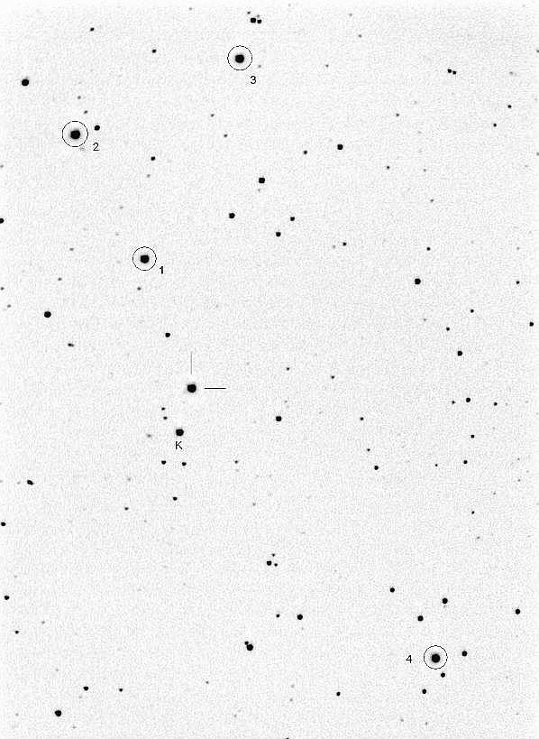
Figure A6. Finder chart showing 4 reference stars. New R-magnitudes for them are listed in the text. FOV = 14 x 19 'arc.
Differential photometry does not easily lend itself for establishing
photometrically correct target star magnitudes. This is because
differential photometry does not implement CCD transformation equations
(or their countpart, Simple Magnitude Equations). Whereas the 4 stars
that I use for "reference" have Rc-magnitudes of 11.046, 9.261,
10.680 and 10.330, I must use 11.09, 9.30, 10.77 and 10.42
in order to produce the correct XO-1 Rc-magnitude of 10.806.
These small differences will be different for every observer, since
every telescope system has a unique response to star color. Every
observer will have to establish their own set of reference star
empirical magnitudes that achieve the correct target star magnitude.
Searching for Other Planets in the XO-1 System
For my longitude (110 W) there are two transit
"windows" for 2006: March 6 to April 3, and May 16 to June 9. I've used
the interval between these windows to monitor XO-1's brightness
stability in order to check the possibility that other planets are in
the same orbital plane as XO-1b and have orbits small enough to transit
XO-1. To date, no convincing candidate fades have been observed.
On April 3 I sold the Celestron that had been used for the previous
year to observe XO-1 transits, and took delivery of a Meade RCX400
14-inch telescope. On April 16 I began observing XO-1 every clear night
for ~2 hours each night. My goal was to either capture an
ingress/egress feature, or produce an average magnitude for the
observing session that was significantly fainter than the average for
other nights. This latter approach to detecting a planet assumes that
the observing session was fortuitously confined to a transit event,
which is possible when observing sessions are shorter than 2.7 hours
(derived in the next paragraph). The observations of nightly-average
magnitude versus date are shown in the next figure (repeated from Fig.
2).
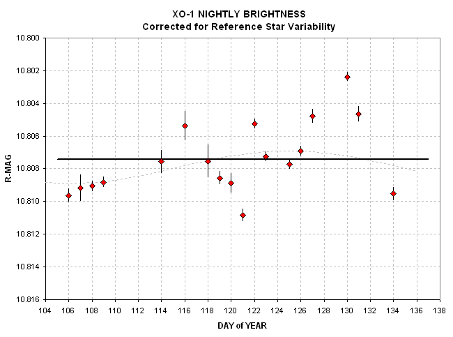 Figure A7
 (Expanded version of Fig. 2, left panel).
Nightly brightness of XO-1 when XO-1b is not transiting for
observing sessions typically 2 hours long. [Meade RCX400 14-inch telescope]
If an additional planet exists that transits the star as seen from
earth, it will necessarily be in an orbit in close proximity to the
Jupiter-mass planet XO-1b. For it's orbit to be stable it will be in a
resonant orbit. The two most likely possibilities are a 2:3 resonance
inner orbit and a 3:2 resonance outer orbit. The inner orbit will be
subject to greater gravitationally destabilizing forces, so the most
likely orbit is a 3:2 resonance outer orbit. The period for the outer
orbit would be 5.91 days (141.9 hours) and the orbit radius would be
1.31 times larger than that of XO-1b. Assuming a tilt of the orbit
plane 2.3 degrees (i.e., inclination 97.7 degrees), the planet would
still transit in front of the star's disk. It's chord length would be
83% of the star's diameter (versus 91% for XO-1b). The transit duration
would be about the same as for XO-1b, 2.74 hours instead of 2.60 hours.
The transit "duty cycle" (fraction of time spent transiting the star)
would be 1.93 %.
What is the feasibility of detecting such a 3:2 resonance planet? Let's
assume that we can detect it if it produces a mid-transit fading depth
of 3 mmag. This corresponds to a solid angle ratio of 14% that of
XO-1b, which corresponds to a diameter ratio of 37%. If XO-1 could be
observed for a continuous 142 hours, and no additional transit was
found, such a planet could be ruled-out. If half that observing time
were accumulated, and assuming there was no phase overlap, then a
non-detection would constitute a 50% ruling-out of such a planet.
So far I've observed XO-1 out-of-transit on 20 dates for a total of 37.5
hours. Assuming these 37.5 hours are not overlapping in phase (for a
142-hour period) this corresponds to ~26% coverage of a hypothesized
3:2 outer orbit resonance planet. In other words, I can't rule-out such
a planet, but the chances of it existing are reduced with every
additional increment of observing time that does not show the star to
be >3 mmag fainter than usual.
There are two candidate fade dates in Fig. 7, DOY = 121 and 134.
Both are of the order 3 mmag, yet I do not beleive either are real and
credible candidates for an actual additional exoplanet transit. I have
three reasons for taking this position: 1) there's
a
positive feature of similar magnitude (DOY = 130) whcih cannot be
explained, 2) the DOY 121 observing session was 3.1 hours long and
the longest transit duration is 2.74 hours for a 3:2 resonance orbit,
and 3) many dates exhibit 2 to 3 mmag differences from the average
that are also much larger than their stochastic SE.
This last point is the most significant one, since it highlights the
fact that there are unexplained systematic errors that are larger than
the stochastic kind. A larger aperture telescope is not necessarily
going to overcome these systemtic errors. Rather, better observing
procedures or image analysis procedures are to be investigated.
There appears to be an auto-correlated variation of XO-1 R-magnitude,
somewhat resembling a monotonic rise in brightness during the 4-week observing interval. The XO-1 brightness is based on
"ensemble photometry" using four reference stars. At least two of these
reference stars is variable at the 5 to 10 mmag level, and I have modeled the variability of all four. Their different
periods will produce apparent XO-1 variations with similar periods, and
I believe that this will eventually explain the systematic deviations
from an average brightness exhibited by XO-1 in Fig. 7. Additional
observations are needed to be sure of this explanation, and to possibly
remove their effect on XO-1 when the variable reference stars are
characterized. More information on this project can be
found at
VariableReferenceStars.

Poisson Noise
"Poisson noise" is related to the fact that a finite number of
stochastic events lead to a "counts" reading from each pixel. Consider
the process of a photon dislodging an electron from a silicon crystal
in the CCD (the "photoelectric effect"). This one event yields one
electron for detection after the exposure is complete. When a pixel is
"read" by electronic circuitry this one electron will contribute to that
pixels count value by an amount that depdends on the CCD gain. For a
SBIG ST-8E CCD, the gain is 2.3 electrons per count (where each "count"
is also called an ADU, or analog data unit). Therefore, the number of
photoelectric events it takes to produce a count of C is n = C / 2.3
for this CCD. Stochastic events have the property that the SE
uncertainty of the total number of events is the square-root of the
number of such events. Thus, when we measure n stochastic events we must state that we have really just measured a value n ± sqrt(n)
events. Since the measurement C is based on C/2.3 events (for this
particular CCD) we must state that we have measured: Counts = C ± sqrt (C/2.3). This fundmental uncertainty is referred to as Poisson
noise. To summarise this, Poisson noise from a bright star is:
Np = sqrt (C / gain)
Np = sqrt (C / 2.3) for SBIG ST-8E.
So far this treatment assumes that there is no noise contribution from
the process of "reading" the CCD ("CCD read noise"), or noise produced
by thermal agitation of the crystal's atoms ("CCD dark current noise"),
or from noise produced by a sky that is not totally dark ("sky
backgound noise"). These are three additional sources of noise in each
CCD reading, and the last two are Poisson themselves since they are
based on discrete stochastic events. These three noise sources are
small when the star in the photometry aperture is bright and the CCD is
very cold (to reduce dark current noise). For this situation we can
state that the star's measured flux (total counts within the aperture
minus a background level of expected counts) will be uncertain by an
amount given in the previous paragraph. If, however, the CCD is not
very cold, which is going to be the case for amateurs without LN2
cooling, the noise will be greater. If there is no star within the
signal aperture then we can calculate that the noise produced by
reliance upon the number s pixels within the photometry signal aperture will be:
Ns = sqrt (s) * Ni
where s is the number of pixels within the signal aperture of
the photometry circles, and Ni is the noise of each pixel. Ni is
calculated as the RMS difference of the counts for the r pixels
within the sky background annulus. If a star is present the total noise
from the signal aperture's count reading is the orthogonal sum of the
star's Poisson noise, Np, and Ns.
Finally, the sky background level cannot be determined with perfect accuracy. The average level of counts from the r pixels contained within the "sky reference annulus" is:
Nr = sqrt (r) * Ni
Since Ni and r have non-zero values, Nr will have a non-zero value. In practice, however, r is so large that Nr is small enough that it can be ignored.
The total noise for a photometry reading (using a SBIG ST-8E) is therefore given by the equation:
N2 = Np2 + Ns2 + Nr2
N2 = C / 2.3 + s × Ni2 + r × Ni2
The signal-to-noise ratio, SNR = C / N. Given that magnitude
uncertainty is 1.085 / SNR, we can state that millimagnitude precision
is:
SE [mmag] = 1085 × sqrt ( C / 2.3 + s × Ni2 + r × Ni2 ) / C
where it is easy to identify the three contributions to uncertainty
associated with the bright star's Poisson noise, the signal circle's
(CCD read, dark current, sky background) noise, and the sky background
reference annulus' (CCD read, dark current, sky background) noise.
Let's insert some typical values into this equation, then calculate SNR
- which is easily converted to "millimagnitude precision."
I'll adopt the following: telescope with 14-inch aperture telescope,
seeing ~4 "arc (FWHM), R-filter, air mass = 1.1, a SBIG ST-8E CCD
cooled to -25 C, plate scale ~1.0 "arc per pixel. The longest exposure
that avoids saturation for XO-1 is ~4 minutes. This is long compared
with the temporal resolution that's desired for exoplanet transists, so
let's calculate noise for 1-minute exposures. A 1-minute exposure
produces C = 225,000 counts. The background noise for each pixel ~11
counts. Good performance is achieved using photometry aperture circles
with radii of 12, 3 and 12 pixels (radius of signal aperture circle,
gap width, sky background annulus width). The number of pixels in the
signal aperture circle is 452 and the number in the sky background
annulus is 1583. The three sources contribute the following noise to SE
[mmag] for 60-second exposures:
1.51 mmag Bright Star Poisson noise
1.10 mmag Signal aperture (CCD read, dark current, sky background) noise
0.03 mmag Sky background annulus (CCD read, dark current, sky background) noise
2.01 mmag Total noise (orthogonal sum)
I measured an empirical noise of 2.23 mmag, so there might be another
component of 0.20 mmag. As described in the next section, scintillation
is a likley candidate.
Since the signal aperture contributes a significant amount to the total
noise, I thought there might be merit in reducing the signal aperture,
thus reducing s × Ni2. However, when I
re-reduced the 2006.03.14 XO-1 transit images using signal
aperture radii of 8, 10 and 12 pixels, the best performance was with
the 12 pixel radius.
Scintillation Noise
At tropopause altitudes clear air turbulence is common, and it causes
stars to "twinkle." (Atmosphereic seeing is degraded mostly by
turbulence near the ground.) Everyone knows that stars twinkle
different amounts on different nights. Twinkling also is greater near
the horizon. Faint stars twinkle as much as bright stars. Planets don't
twinkle as much as stars.
These common facts are helpful in understanding what to expect for
attempts to monitor the brightness of a star that is undergoing an
exoplanet transit. For example, the fact that planets don't twinkle
means that a reference star's scintillation (another word for
twinkling) will be uncorrelated with the target star's scintillation.
This is unfortunate, for it means that a differential photometry
analysis that uses one reference star will increase the target star's
brightness variations due to scintillation by ~41% (i.e., root-2 more
variation). Using many reference stars reduces the effect of
uncorrelated reference star scintillation back to where it is dominated by just the target star's scintillation. It also can be
stated that there's no need to chose reference stars that are near the
target star to reduce scintillation, since essentially all correlation
is lost with angular distances of 10 "arc (a typical planet angular
diameter).
Andy Young conducted a classic study of scintillation in the 1960s
(Young, 1967, 1974). He studied it's dependence upon telescope
aperture, air mass, observatory altitude and exposure time. His
equation relating all these parameters is:
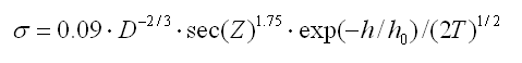
where sigma = fractional intensity RMS fluctuation (scintillation), D =
telescope diameter [cm], sec(Z) = air mass, h = observatory site
altitude above sea level [m], h0 = 8000 [m], and T = exposure time [sec].
For my site, and specifically for the 2006.03.14 observations of XO-1,
for which I have measurements to compare with theory, I calculate
expected typical scintillation using the following input:
D = 35.6 cm
air mass = 1.1
h = 1420 meters,
T = 60 seconds,
The predicted scintillation using this input is 0.82 mmag.
As stated in the previous section Poisson and other CCD-related noise
accounted for only 2.01 mmag of an empirically measured 2.23 mmag noise
for XO-1 on the night of 2006.03.14 (near zenith). The missing 0.20
mmag is likely to be due to scintillation. Why, you mihgt ask, was the
missing noise source as small as 0.23 mmag when the scintillation
equation predicts 0.82 mmag. Recall, scintillation varies from night to
night, and the equation is for "typical" scintillation fluctuations. On
the night in question a high pressure was overhead, and the winds at
ground level were uncommonly low (being zero mph for hours at a time).
I conclude that I was lucky with good weather for the 2006.03.14
observations and my scintillation noise was ~0.23 mmag.
To summarize, the measured precision of 2.23 mmag per 60-second image is close to the
theoretical limit of 2.17 mmag. The noise sources for a 60-second image
using my telescope system are summarized in the following table:
NOISE BUDGET FOR 14-INCH
TELESCOPE
(Assuming Target Star is at 12% of Full-Scale and Ensemble Photometry Using Many Bright Stars)
Noise Value
|
Noise Source
|
1.51 mmag
|
Bright star Poisson noise (12% of full scale, flux ~225,000 counts)
|
1.10 mmag
|
Signal aperture (CCD read-out, dark current, sky background) noise
|
0.82 mmag
|
Scintillation (typical)
|
0.03 mmag
|
Sky background annulus noise (dark current, sky background, CCD read-out)
|
2.17 mmag
|
Total SE for 1-minute exposure
|
In conclusion, to achieve that "gold standard" 1.0 mmag SE for XO-1,
using a 14-inch telescope and ensemble photometry that includes a
reference star 1.53 magnitudes brighter than XO-1, it will be necessary
to average the results from at least four
1-minute exposure images.
Larger apertures should be able to achieve millimagnitude results more
easily, although their exposure times will have to be shortened to
avoid saturation. It should be each observer's responsibility to use
the concepts described here to calculate their own optimum observing
strategy.
Transit Schedule for the Remainder of 2006
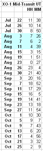
Figure A8. Predicted mid-transit times for the remainder of
2006. For ingress (contact 1) subtract 1.5 hour, for egress
(contact 4) add 1.5 hour. Blue-shaded dates are ideal for Western
USA. Later dates are observable from longitudes eastward of Western
USA. Assumed period is3.941534 days (as given in the ApJ article); actual times may be a few minutes earlier.
After the Oct 25 transit XO-1 is too close to the sun for favorable
viewing for the remainder of 2006. For the Western USA there are only 3
dates when a complete transit can be observed (Aug 3, 7 and 11).
Related Links
Astrophysical Journal article:
http://xxx.lanl.gov/abs/astro-ph/0605414 (Abstract)
http://arxiv.org/PS_cache/astro-ph/pdf/0605/0605414.pdf
Co-author sites:
http://hubblesite.org/news/2006/22 (Peter McCullough, STScI)
http://www.media.rice.edu/media/NewsBot.asp?MODE=VIEW&ID=8563&SnID=692431138 (Johns-Krull, Rice University)
http://www.bu.edu/phpbin/news/releases/display.php?id=1136
(Kenneth Janes, April Pinnick & Paul Howell, Boston University)
http://www.ifa.hawaii.edu/info/press-releases/extrasolar_planet/
(Peter McCullough & James
Heasley, STScI; Bill Giebink, Les Hieda,
Jake Kamibayashi, Daniel O’Gara, and Joey Perreira, Univ. Hawaii staff)
http://www.cbabelgium.com/ (Tonny Vanmunster)
http://ronbissinger.home.comcast.net/favorite.htm (Ron Bissinger)
http://www.howell-ltd.com/Astronomy/html/exoplanet.html (Paul Howell)
My other exoplanet transit observations:
Observations of other XO-1 transits
Modeling Size of Planet XO-1 (an amateur's version)
Exoplanet transit
observations of TrES-1
Exoplanet
Transit Observations of HD209458
HD37605 exoplanet
(possible transit system)
HD74156 exoplanet
(possible transit system)
IL Aqr exoplanet reference
stars
Mscellaneous Related Web Sites
Arto Oksanen's first-ever amateur exoplanet light curve
Sky & Telescope article on XO-1
All-sky photometry using Simplified Magnitude Equations
Draft of an old exoplanet observing tutorial
Bruce's Astrophotos (with many other links)
Resume
References
Landolt, A. U., 1992, AJ, 104, 340
McCullough, P.R., Stys, J. E., Valenti, J. A., Fleming, S. W., Janes, K. A. and Heasley, J. N., 2005, PASP, 117, 783.
McCullough, P.R., Stys, J. E., Valenti, J. A., Johns-Krull, C. M.,
Janes, K. A., Heasley, J. N., Bye, B. A., Dodd, C., Fleming, S. W.,
Pinnick, A., Bissinger, R., Gary, B. L., Howell, P. J., Vanmunster, T.,
(in press), Ap. J., "A Transiting Planet of a Sun-like Star"
____________________________________________________________________
This site opened: May 11,
2006. Last Update: July 17,
2006