EXOPLANET TrES-1 TRANSIT OBSERVATIONS
Bruce L. Gary; Hereford, AZ
This
web page was created in 2004 and discontinued a year later. Its
original purpose was for the purpose of data exchange with other
TrES-1 observers and data analysts at a time when a group of amateurs
suspected a "brightening" just outside the transit feature. Such a
brightening after egress (and before ingress) could be produced by
forward scattering of a ring system around the TrES-1 hot Jupiter,
TrES1b. Since it might be usefual in serving as a tutorial
for exoplanet observing and analysis procedures I will leavit up for
awhile (this is 2007.11.22). For a more comprehensive and up-to-date
web page of amateur observations of TrES-1 go to http://brucegary.net/AXA/TrES1/tres1.htm
Links internal to this web page:
Transit of
2005.04.26
Schedule for 2005
Combined
data light curve
Test Observations on a
non-transit night
2004 October 08
transit (ingress)
2004 October 02 transit
(ingress & mid-transit)
2004 September 23
transit (mid-transit & egress)
All BLG Data
Equipment and
Observing/Reduction Procedures (tutorial for exoplanet observing)
General
Introduction to TrES-1 Star Field
Links to
text
data files
Links to
other relevant web sites
Transit of 2005.04.26
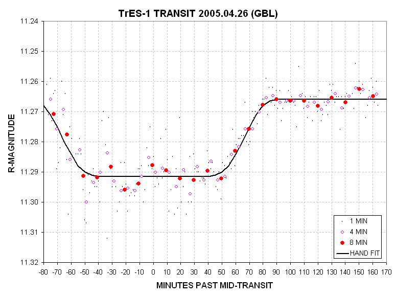
Figure 1 Transit of April 26, 2005.
Individual 1-minute exposures are shown with dots, while 4-minute
and 8-minute averages are shown using purple and red symbols. A
hand-fitted line is shown with symmetry about the predicted transit
time. The first observations were made at an elevation of 12
degrees and the last data were made at an elevation of 54 degrees.
Ensemble photometry used 7 reference stars that surrounded TrES-1. The
RMS scatter about the hand-fitted trace is is 2.9 mmag for 4-minute
average data and 2.1 mmag for the 8-minute data.
Based on this data I no longer believe that TrES-1 has a bump upon
egress, and I'm discontinuing my observations of this object.
These observations were made with a red filter. The flat field frame
was a median combine of 25 individual flat frames with maximum counts
between 25,000 and 32,000, all with exposures between 1 and 10 seconds,
and they were made with a double T-shirt aperture cover at sunset. The
dark frame consisted of 27 1-minute exposures, median combined, made
with the CCD at the same temperature as the TrES-1 observations (-25
C). A SBIG AO-7 tip/tilt autoguider was used, with an exposure time of
0.2 seconds using a star with a V-magnitude of 10.6. A dither parameter
of 1 assured that each image was randomly offset from a nominal
location by approximately 3 pixels. An observing sequence was
employed that specified 16 1-minute exposures with a 5-second settle
time before each exposure (to allow the AO-7 to re-center the autoguide
star). Processing was done using MaxIm DL's photometry tool, with
aperture settings of 11, 3 and 9 pixels. The FWHM for each 1-minute
exposure ranged from 3.6 "arc to 7.5 "arc (the larger values were
confined to the 12 - 20 degree elevation region). A spreadsheet
analysis showed no correlation of TrES-1 departure from a regional
average with FWHM.
Measurement precision improves with elevation angle. The following
graph shows precision versus air mass for the three averaging times:
1-minute, 4 minutes and 8 minutes.
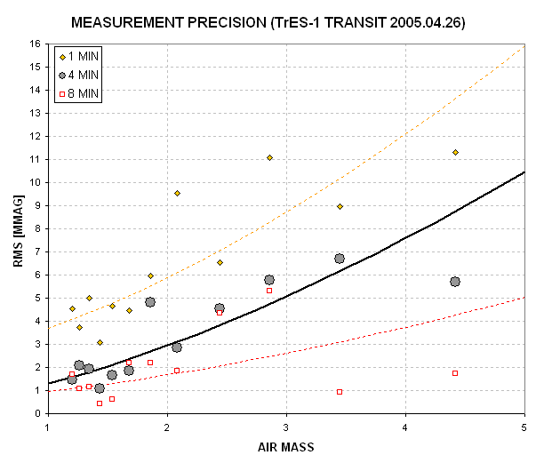
Figure 2 Measurement precision versus air mass for three
averaging times. The fitted traces suggest that for air mass =1.5 the
measurement precision is ~5, ~2 and ~1.3 milli-magnitude for averaging
times of 1, 4 and 8 minutes.
Ensemble photometry offers the opportunity of estimating the magnitude
of RMS variation a suspect variable object should exhibit based on its
brightness. For example, the TrES-1 observations were reduced using 7
reference stars and 7 check stars. Thus, 14 non-variable stars provided
an estimate of expected variability due to scintillation and stochastic
noise as a function of brightness, and TrES-1 exhibited much greater
variability than the expected amount, as shown in the following figure.
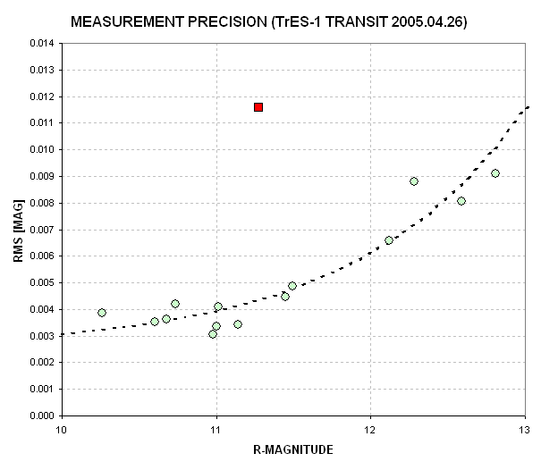
Figure 3 Measured RMS versus brightness for the 7
reference stars and 7 check stars (green circles) and TrES-1 (red
square). The dashed trace is a model for precision that involves a
constant (i.e., scintillation) and a term that is inversely
proportional to star flux (stochastic component). The RMS is for
magnitude readings from 1-minute exposures.
If TrES-1 were non-varying it would have exhibited an RMS
variation during the 3-hour observing period of ~0.004 magnitude, based
on the variability of the reference and check stars. Instead, it had an
RMS variation about its average of 0.0115 magnitude. Presumably, the
transit light curve in Fig. 1 is "real."
The following image shows which stars were used for reference.
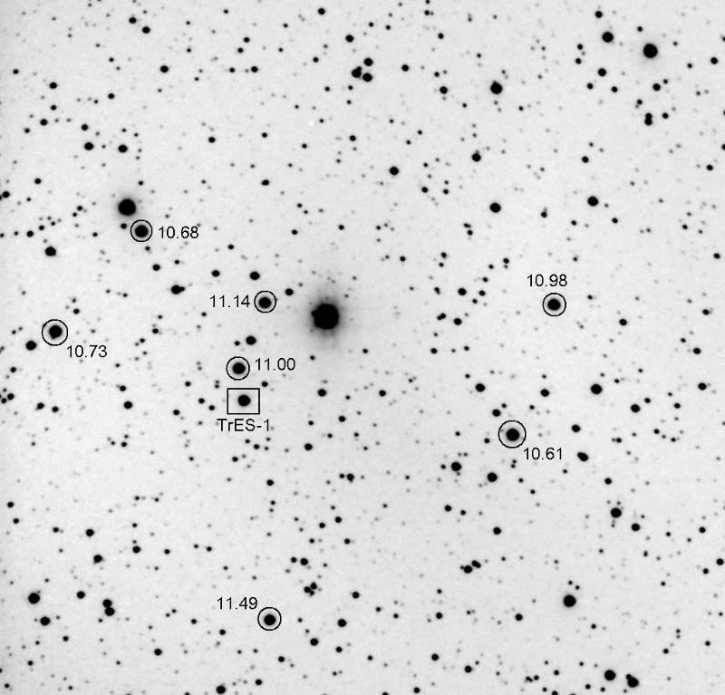
Figure 3 Image of TrES-1 region showing 7 reference
stars used to perform the ensemble photometry for this night. All
magnitudes are for R-band. North up, east left; FOV = 16.4 x 15.7 'arc.
[Total exposure time is 115 minutes.]
Schedule
for 2005
[This section was prepared before I decided to discontinue
exoplanet transit observations. I leave it here because it might be
useful for others wanting to schedule observations for their site.]
Every observer should consider identifying which TrES-1
transits can be usefully observed at their site. I will present
graphical and table representations of what I have determined for my
site in Southern Arizona. Differences in longitude are more critical
than latitude for making these identifications. There are two factors
to consider when assessing a specific transit's observability: 1)
TrES-1 elevation above the horizon, 2) Sky darkness (sun's elevation
below the horison and the moon's phase and proximity to TrES-1). First,
I will show a graphical representation of these factors.
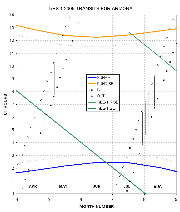
Figure 4 UT times for sunset (blue) and sunrise
(orange) are shown versus date. Dotted lines are used to indicate when
the sky is dark enough for observations to be made (offset 45 minutes
from sunset and sunrise). UT times when TrES-1 rises and sets
through 20-degree elevation are shown with green lines. The
TransitSearch times for ingress and egress are shown with small open
squares. Vertical lines join ingress to egress times for those transits
that occur when it is dark and when TrES-1 is high in the sky.
For all of the transits identified as observable in the graph the moon
is below the horizon. This is fortunate for observers in the Western
United States. Europeans will have a completely different set of
circumstances, and may in fact be bothered by the moon in 2005.
Here's a table of the 9 transits that I have identified as observable
from Southern Arizona for 2005.
|
DAY OF WEEK
|
UT DATE
|
INGRESS UT
|
EGRESS UT
|
1
|
Sun
night
|
May
2
|
6:55
|
9:31
|
2
|
Wed
night
|
May
5
|
7:38
|
10:14
|
3
|
Sat
night
|
May
7
|
8:21
|
10:58
|
4
|
Thu
eve
|
Jul
29
|
3:50
|
6:27
|
5
|
Sun
eve
|
Aug
1
|
4:33
|
7:10
|
6
|
Wed
eve
|
Aug
4
|
5:16
|
7:53
|
7
|
Sat
night
|
Aug
7
|
6:00
|
8:37
|
8
|
Tue
night
|
Aug
10
|
6:43
|
9:20
|
9
|
Fri
night
|
Aug
13
|
7:26
|
10:03
|
For egress only observing (i.e., foresaking ingress) there are
at least 4 more observing opportunities: April 26 and 29, and July 23
and 26 (UT).
Combined Data Light Curve
The following figure shows light curves for the TrES-1 data that
has been made available to me. They have undergone small adjustments
for temporal trends and time shifts (see details for
details). Tonny Vanmunster (VMT) has measurements
for the dates 2004.09.01 (abbreviated hereafter as "4901") and
2004.09.04 (abbreviated as "4904"). My observations (GBL) are for the
dates 2004.09.23 ("4923"), 2004.10.02 ("4A02") and 2004.10.08 ("4A08").
Tonny's data is high quality, and mine are not as good but still
useable. Here's a plot of sliding boxcar averages of our data.
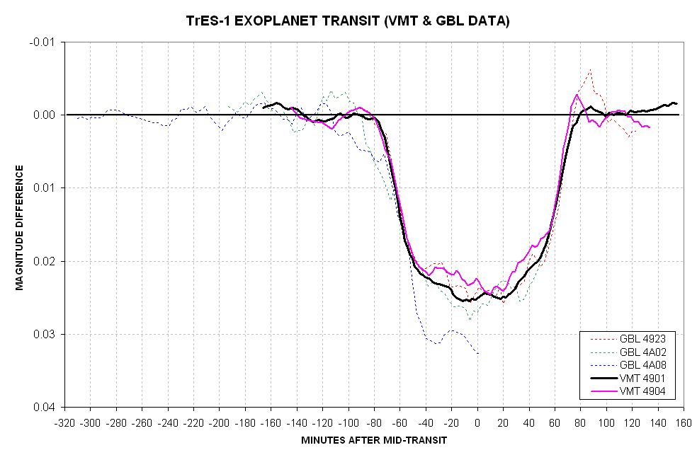
Figure 5. Magnitude measurements of TrES-1
transits made by Tonny Vanmunseter (VMT) and the author (GBL) are
plotted with respect to "time after mid-transit" with magnitude offsets
that achieve zero away from transit. The VMT data with a sample
interval of 2.4 minutes have been smoothed with a 24-minute "sliding
boxcar filter"and adjustments were made for temporal trends and slight
timing offsets (to achieve symetry about the predicted mid-transit
time). The GBL data have a sampling interval of 3.1 minutes, a
22-minute sliding boxcar averaging interval, and two of the three data
sequences have been adjusted for temporal trends and one was adjusted
for a time offset. The VMT 2.4-minute data exhibit an RMS scatter about
their average trace of 1.7 and 2.8 milli-magnitude (for 4901 and 4904).
The GBL 3.1-minute data exhibit a RMS scatter about the average trace
of 4.5, 4.5 and 4.8 milli-magnitude. The trace for "GBL 4A08" goes
below the others during transit when high air mass conditions were
encountered (no temporal trend correction was attempted for this data
sequence).
Tonny Vanmunster's measurements are much more precise than mine,
so any "features" in his light curves should be viewed as more
credible. The purpose for my 4A08 observations was to evaluate
"bumpiness" during a time when no transit was expected, in order to
know whether any "bumps" during transit should be taken seriously. My
non-transit light curve data for 4A08 "wander" about zero with an
amplitudes of ~1.5 milli-magnitude. I will take the position that any
features in my light curves that are smaller than 2 milli-magnitude
should be disregarded as mere stochastic and systematic wander. In
addition, for the 4A08 data sequence I will assume that starting at
-110 minutes there is a systematic fading trend that amounts to ~0.005
magnitude that is not real, and for which a plausible explanation is
that some effect related to increasing air mass caused this fading
trend. Thus, the 4A08 "soft shoulder" during ingress is to be
disregarded.
Considering only the GBL data for now, and adopting the guideline that
stochastic and systmatic error wander can be expected to exist at the 2
milli-magnitude level, I conclude that there are two candidates for
real anomalies that might be attributable to TrES-1: 1) an ingress
brightening of "GBL 4A02" at -110 minutes, and 2) an egress brightening
of "GBL 4923" at about +90 minutes. I'll return to a discussion of
these features later.
Considering the VMT data, there is insufficient coverage away from
transit to allow the same evaluation of stochastic and systematic error
wander (in the same way that this was done for "GBL 4A08"). VMT data
have much better stochastic properties, but it is difficult to assess
the magnitude of VMT systematic error wander. One approach is to
compare the two VMT curves, and assume they have the same systematic
error wander properties and also assume that the TrES-1 light curve is
the same for each transit. If this were done then the inferred VMT
systematic error wander would be ~1.0 milli-magnitude (slightly better
than attributed to GBL). Under this assumption the VMT data show only
one anomaly: an egress brightening of "VMT 4904" at about +80 minutes.
With only this limited set of data, from only two observers, the case
for a brightening before ingress and after egress is unconvincing for
me. Let's consider these light curves under the assumption that the
TrES-1 light curve is the same every transit. The following graph shows
my best estiamte of this combined data light curve.
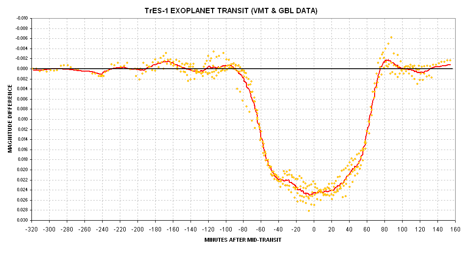
Figure 6. Average of all VMT and GBL data (adjusted
for temporal trends and time shifted). This light curve is based on data points
that are themselves temporal averages (24 and 22 minutes) so there is
no possibility for the presence of shorter timescale features.
If it is assumed that every transit has the same light curve then this
last figure is an approximation of it. Any egress
brightening for such a light curve would have an amplitude of ~2
miili-magnitude.
It is my personal opinion that this set of data cannot be used to argue
strongly for or against the presence of anomalous features in the
TrES-1 transit light curve. This data set is limited to just two
amateur observers (with AAVSO observer codes VMT and GBL). The
TransitSearch group is in possession of a much larger data base for the
TrES-1 transits, and Ron Bissinger has performed a very good analysis
of it. When a web site for that analysis is available I will put a link
to it here.
Test
Observations on 2004 November 04 (Non-Transit Night)
To satisfy my curiosity I observed TrES-1 for 3.4 hours on a
non-transit night to see what level of variations would be observed
using the same observing hardware configuration, observing technique
and the same data reduction procedure that was used for the transit
observations. Here's what I got for a light curve.
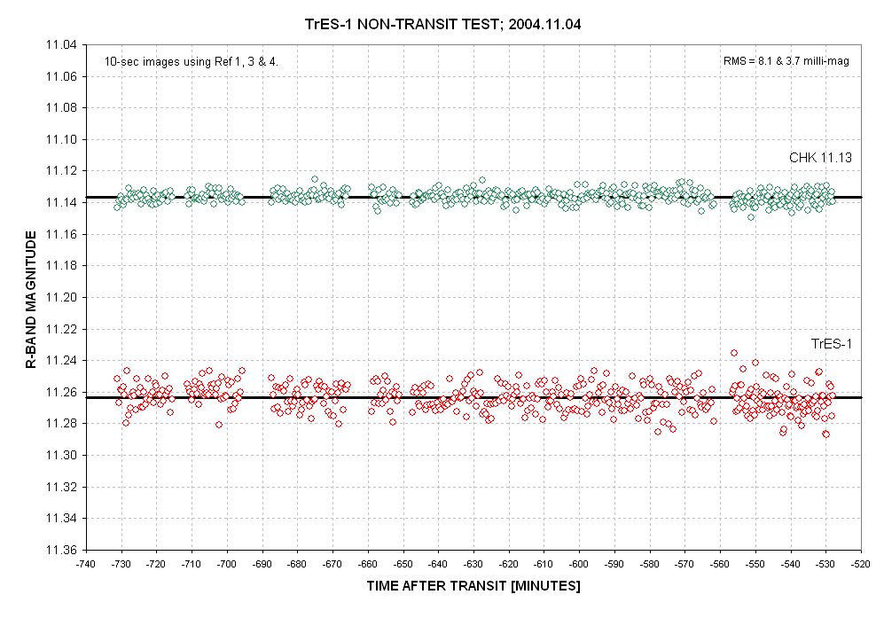
Figure 7. Measured R-magnitudes on a non-tranist
night for TrES-1 (red) and a check star
(green) using same hardware and procedures as during the transit
nights. Three stars served as reference ("comp").
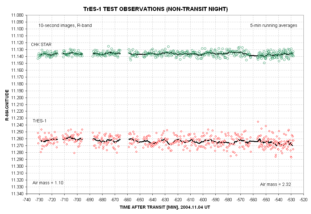
Figure 8. Light curve plot of same data as in
previous figure. A 5-minute
running average is shown.
The observations began with air mass = 1.10 and ended when airmass =
2.32. The RMS deviations from the running average increase with air
mass from 3.07 to 3.84 milli-magnitude for the check star and they
increase from 6.85 to 8.58 milli-magnitude for TrES-1.
TrES-1 exhibits an RMS variation about the 5-minute running average
trace that is greater than for the check star. For example, at low air
mass the two RMS values are 3.07 milli-magnitude (check star) and 6.85
milli-magnitude (TrES-1). The RMS fluctuations are in the ratio 2.22
instead of the expected 1.12 (based on brightness ratios). I don't
understand this.
The 5-minute average trace for the check star exhibits a range of
variation of ~6 milli-magnitude, whereas the range of variation for
TrES-1 is about 10 milli-magnitude. Clearly, for my transit
observations features similar to those in the above figure should not
be believed. Specifically, a 5-minute feature with an amplitude of 2
milli-magnitude is too subtle for me to detect with one observing
session (especially when TrES-1 is at a high air mass).
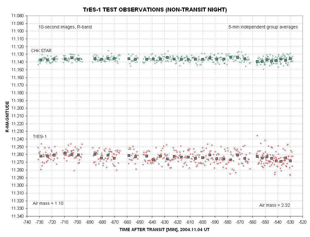
Figure 9. Light curve plot of same data as in
previous two figures. 5-minute
independent group averages are shown.
The 5-minute group averages for the check star exhibit an RMS about
their ensemble average of 0.88 milli-magnitude at low air mass to 1.56
milli-magnitude at high air mass. For TrES-1 the RMS deviations from
the ensemble group average is 2.25 milli-magnitude at low air mass and
2.42 milli-magnitude at high air mass.
The check star 5-minute independent group average of 0.88
milli-magnitude at low air mass agrees well with the value expected
from the 10-second individual image RMS of 3.07 milli-magnitude (0.89
milli-magnitude). The check star's high air mass RMS is slightly higher
than the expected value, 1.56 versus 1.11 milli-magnitude. I interpret
this to be evidence that high air mass observing conditions produce
systematic errors that wander by amounts greater than the stochastic
uncertainty (for my system). This appears evident in the check star's 4
milli-magnitude "fade feature" at about -575 to -555 minutes. TrES-1's
5-minute independent group averages undergo a greater fluctuation than
the check star, as predicted from their greater RMS for individual
10-second images. The TrES-1 5-minute groups exhhibit approximately the
expected RMS values for both low and high air mass, being 2.25 versus
2.00 milli-magnitude for low air mass and 2.42 versus 2.48
milli-magnitude for high air mass.
Using the 5-minute independent data groups it is possible to predict
the level of features that can be expected to appear during a real
transit event, assuming stochastic SE and systematic wander
characteristics are the same both observing nights. TrES-1 and the
check star tell the "same story": we should expect to see non-real
10-minute features with amplitudes ~2 milli-magnitude at low air mass
and ~3 milli-magnitude at high air mass. Given the better stochastic
behavior of the check star (than TrES-1) these systematic error
wanderings will be more apparent for a star that is stochastically
well-behaved (like the check star was). For a star with poorer
stochastic behavior (like TrES-1) the systematic error wandering will
be less apparent (although it is approximately the same as for the
stochastically well-behaved check star).
Another way to approach the question of whether to believe features in
an exoplanet light curve is to perform a transit simulation using
non-transit observations. This is done in the next two figures.
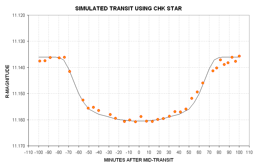
Figure 10. Simulated light curve using
measurements of a nearby check star and adjusting them using a
hypothetical transit light curve with TrES-1 properties.
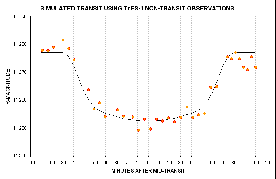
Figure 11. Simulated
transit light curve using TrES-1 non-transit observations and adjusting
them using a hyothetical transit light curve with TrES-1 properties.
The two figures, above, were created from the non-transit measurements
of 2004.11.04 by applying a hypothetical transit light curve shape
adjustment to the non-transit observations. These plots show what can
be expected when observing a transit. If the "eye" detects features in
these light curves then the "brain" should intervene and say "no,
they're not real; they're roduced by systematic error wander." Indeed,
in the second of these simulated transits (based on TrES-1 non-transit
observations) note the apparent "bump" before ingress. There is no
corresponding brightness bump after egress, and in fact there appearsto
be a fading after egress. The first of these "features" must be
attributed to systematic error wander and the latter feature may be due
to wander associated with high air mass.
The "message" from this simulation is that instrumental anomalies
having amplitudes of ~3 or 4 milli-magnitude should be expected from an
observing system (and analysis procedure) used by the author of this
web page. If other observers want to argue for the "reality" of their
anomalies then it may be instructive for them to conduct a simulation
using non-transit observations similar to what I have described on this
web page. As an alternative light curves obtained by several observers
could be combined to see if all of them, or most of them, show the same
anomalies. That analysis will be performed for the TrES-1 2004
October/November observations by Aaron Price (AAVSO) in the near
future.
In the above two figures notice the better "behavior" of the check star
compared with TrES-1. As stated earlier, I do not undersxstand why
TrES-1 has a higher
stochastic SE than the check star (whose brightness is only 12%
greater). It may have something to do with nearby faint stars with PSFs
whose edgtes wander in and out of the signal aperture or sky reference
annulus. Or maybe the three reference stars were better located for
removing flat field errors (i.e., the reference stars "surrounded" the
check star better than TrES-1).
This exercise illlustrates some of the considerations and supporting
observations that can lead to improved understanding and performance in
exoplanet transit monitoring.

2004
October 08 (ingress)
This section (and the following ones) describe my TrES-1 transit
observations.
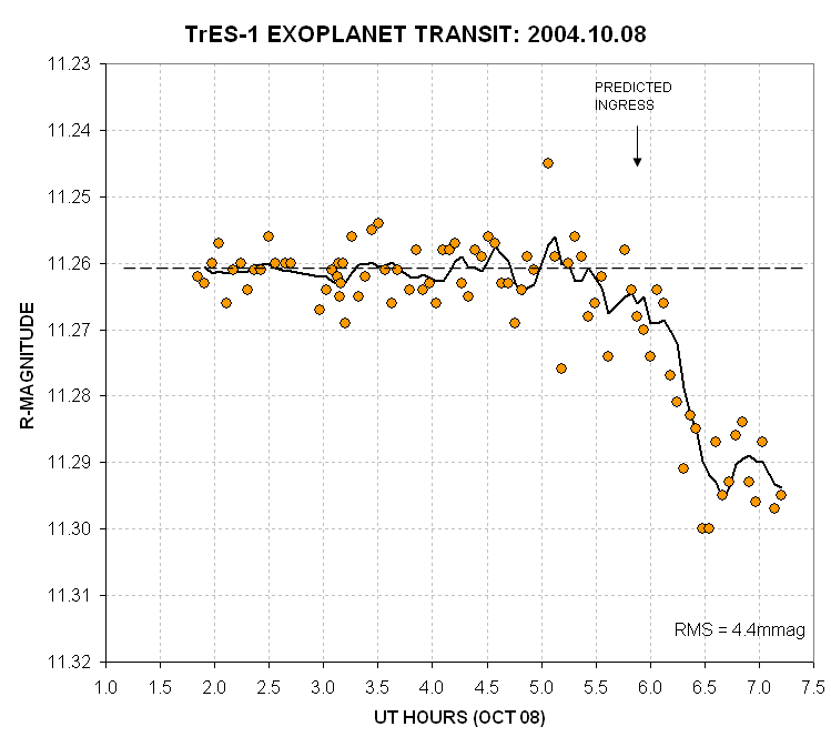
Figure 12. Each datum is from a median combine of
five 30-second exposures, and represents an observation taken within a
200-second observing window (which allows for image download time). A
photometric R-band filter was used. The first observations were made
just after transit and the observations end when the elevation was 19
degrees (m=3.1). Two "outliers" occur (near 5.0 hours) when I was
negligently changing the focus setting. The residuals from an average
trace have an RMS = 0.0038 magnitude (excluding the two "outliers").
2004
October 02 (ingress & mid-transit)
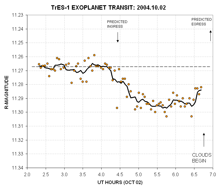
Figure 13. Each
datum is from a median combine of ten 10-second exposures, and
therefore represents an observation taken within a 190-second window.
An R-band filter was used. The
residuals from an average trace have an RMS = 0.0044 magnitude
(excluding one "outlier").
2004
September 23 (mid-transit & egress)
This is my first observation of TrES-1. I used a V-band filter and
unguided 10-second exposures. After 5 sequences of 10 exposures I
re-centered the telescope so that the exoplanet was at the center of
the FOV.
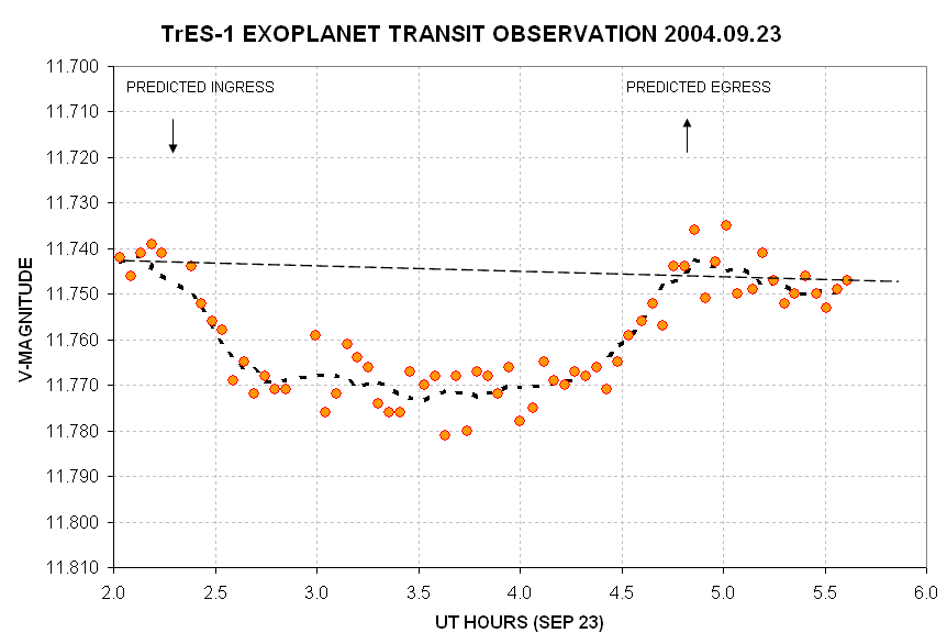
Figure 14. Observations of September 23, 2004 (UT). A
V-band
filter was used for 10-second exposures, median combined in groups of
10. Each datum is therefore from a total exposure of 100 seconds
occurring within a 180-second observing window (which allows for image
download time). The
RMS residual from the average trace is 4.7 milli-magnitude. A "meridian
flip" was required at ingress which accounts for the slight gap at that
time (never buy a German equatorialmount for exoplanet work). The early
data are near zenith whereas the late data correspond to 50 degees
elevation.
In this light curve there appears to be a "bump" at
egress, or maybe a dip after egress. This bothered me until I saw other
light curves showing a similar bump/dip feature after egress. That's
when I alerted the TransitSearch discussion group (September 29) about
this interesting anomaly (the discussion group's first "post"). Greg
Laughlin (who set-up the TransitSearch discussion group) received an
e-mail from Joe Garlitz pointing out the
same feature. I suggested that maybe the TrES-1b planet had a satellite
in a synchronous orbit that produced a second smaller "transit"
after the planet had completed its transit, but David Blank
discounted that idea using stable orbit theory, and suggested that
rings might be a better explanation (October 2). On the same date Ron
Bissinger called attention to a presentation at the 2003 AAS DPS
meeting in Monterey by Barnes and Fortney describing what a ringed
planet transit would look like (also described in Sky and Telsecope, January, 2004).
Rings have remained the best candidate explanation so far.
All BLG Data
There is merit in combining data with
comparable quality to look for patterns before combining data with
disparate temporal sampling and quality for the same purpose. All of my
data have approximately the same temporal sampling, were taken with the
same instrument, processed using the same procedure, and they exhibit
approximately the same RMS residuals with respect to an average trace.
Hence, these three data sets are suitable for combining into one larger
data set. The following graph is a superposition of the three data sets
shown in the above sections.
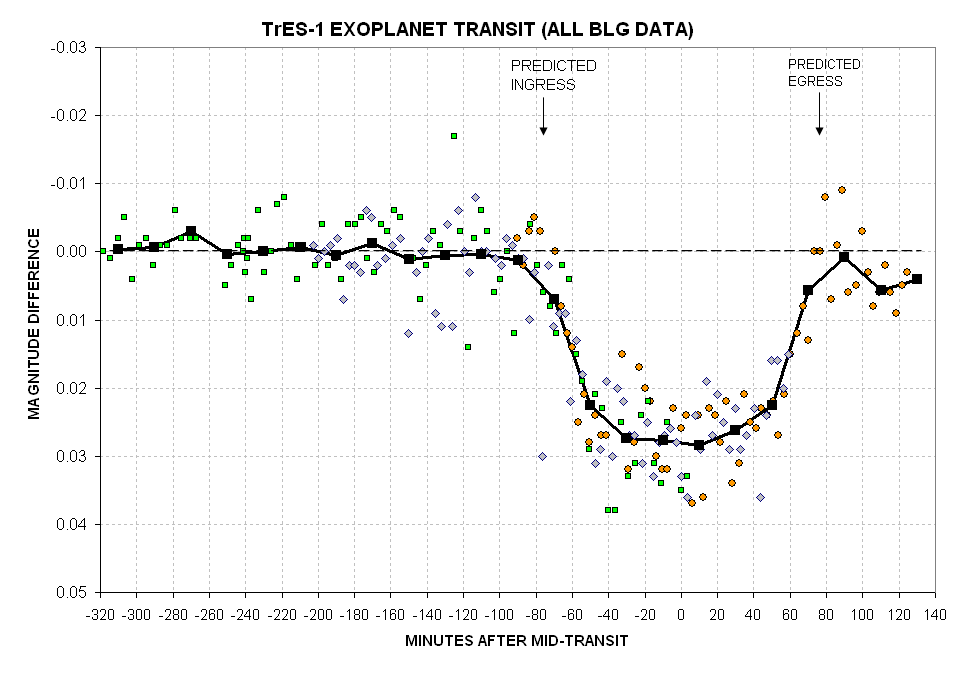
Figure 15. All data in the previous light curve
graphs
are combined in this graph. The average trace is for 20-minute chunks
of data. The vertical offsets were subjectively chosen.
This figure suffers from a lack of data near egress. Only three dates
of ingress data are shown, and there are no unusual departures from a
smooth ingress shape in this graph. This does not rule out the presence
of unusual ingress shapes for other transits but it argues against a
persistent ingress shape having a temporal scale of 20 minutes. The
egress anomaly could be viewed as a dip following egress, with
presumably a return to a pre-transit brightness past the dip. The
argument for a dip instead of a positive bump in brightness is based on
the way I chose an offset for this date's data; I chose an offset that
provided best agreement with data from the other two dates (mid-transit
and pre-ingress). However, using just this set of data it
would be foolish to believe in an anomaly near egress. The egress data
from 2004.09.23 were at lower elevations than the earlier data so it is
possible that extinction effects compromise data quality near the end
(at egress).
Using just my data I would not take a
position concerning the existence of ingress or egress shape anomalies.
It will be necessary to combine data sets from many observers to arrive
at some concensus, and this is what Ron Bissinger is currently doing.
One additional comment can be made from
inspection of this figure. The average trace appears to exhibit a
precision of 0.001 magnitude, based on the pre-ingress data. Averaging
seems to have worked its magic, in this case, without apparent
degradation by unknown systematic errors.
Equipment and Observing/Reduction Procedures
My location is Southern Arizona, 90 miles SSE of Tucson (near the
border with Mexico). The site is on the western edge of a 15-miles wide
valley (San Pedro Valley), with the Huachuca Mountain Range a few miles
to my west. My altitude is 4660 feet, and my coordinates are 110.2378
West, 31.4522 North. I use a Celestron CGE-1400
(14-inch aperture) Schmidt-Cassegrain telescope configured for prime
focus using a a HyperStar (Starizona product) transition lens. The
f-ratio was
1.86. My CCD camera is a SBIG ST-8XE and I use a SBIG CFW-8 filter
wheel with photometric filters. This configuration produces an image
scale of 2.81
"arc/pixel and the FOV was 72x48 arc. Since the "atmospheric seeing"
typically is 2.5 to 3.0 "arc (FWHM), the prime focus configuration
point-spread function has a FWHM of ~7.5 "arc. The telescope is located
in a sliding-roof shed 50 feet from my house, and it is controlled
using 100-foot buried conduit cables from my house office. The MPC has
assigned my observatory an "observatory code" of G95 and name "Hereford
Arizona Observatory."
I use MaxIm DL 4.0 to control the telescope and camera. A typical
observing night starts with dusk sky flat frames for each filter to be
used. I place a "Double T-shirt Cover" on the aperture and point to
zenith for flat frame exposures. This assures that no stars show up on
the flat frame images. Exposure times longer than 1 second are used
(dark frame
subtracted), with exposure times chosen so that the maximum count is
under 40,000 to assure that saturation effects will be small (my CCD is
non-ABG). All dark
frame images for a given filter are then averaged. The CCD cooler is
then set to a value of about -18 C, and during cool down the telescope
pointing and focus is verified near the region of interest.
Observations of the exoplanet are preceded by a focus check and a
star field position placement that provides a suitably bright star on
the autoguider chip. It is common practice for exoplanet observations
to use a filter, such as V or R, in order to minimize extinction
effects as the airmass changes during along observing session. The
exoplanet is almost always placed at the center of
the FOV since with the prime focus configuration the autoguider chip
almost always has suitably bright stars present. My goal is to maintain
this placement of the star field with respect to the main chip for the
entire duration of the night's exoplanet observations. This is an
important
observing goal since errors in the flat field are an important source
of systematic changes in exoplanet brightness. Exposure times for the
exoplanet images are kept short enough that none of the reference stars
produces maximum counts that exceed 40,000. For TrES-1 and R-band this
exposure time could be as high as 60 seconds for my system, but so far
I have used only 30-second exposures. I use MaxIm DL's "sequence"
observing feature to take many sets of 10 "light" images and one "dark"
image.
For data analysis I also use MaxIm DL, including its Photometry Tool
for photometric analysis of groups of images. I manually load 5 images
at a time, calibrate them (flat field and dark), and save the median
combined (or sigma-clip combine) image. I am very wary of cosmic ray
effects creeping into light curve analyses, so I always use median
combined (or sigma-clip combined) images for my photometric analyses.
After several groups of 5 raw/calibrated images have been processed to
produce "clean" images I perform a photometric solution for several
clean images using the MaxIm DL Photometric Tool. The exoplanet
"object" is chosen, and several "reference stars" are also chosen and
their magnitudes are entered in to the Photometric Tool. The choice of
signal aperture radius, gap width and sky reference annulus width are
important, and for the prime focus configuration I usually use 5, 2 and
4 pixels. The stars typically have FHWM = 2.7 pixels, so use of 5
pixels for the aperture radius is "conservative" in the sense that for
images when the FWHM is larger than for other images there will be
minimal effect on the "intensity" reading. Occasionally a star field
has interfereing stars near a reference star (or the exoplanet) and
this requires a different choice for aperture/gap/sky reference. The
Photometric tool creates a CSV-file containing a Julian Day time tag
and magnitudes for the object and reference stars. These are imported
to an Excel spreadsheet and processed in a straightforward manner.
Checks are usually performed to validate constancy of the reference
stars with respect to each other, which is another way of using these
stars for the role of "check stars."
For those wanting a more complete tutorial on exoplanet observing
try http://brucegary.net/ILAqr/
General
Introduction to TrES-1 Star Field
The exoplanet system TrES-1 is located in the constellation Lyra at
RA = 19:04:10, Dec = +36:37:57. The star, TrES-1a, has a V-magnitude of
11.74. Several non-variable stars are nearby with approximately the
same brightness and these can serve as reference stars. Here's a wide
field image of the TrES-1 star field:
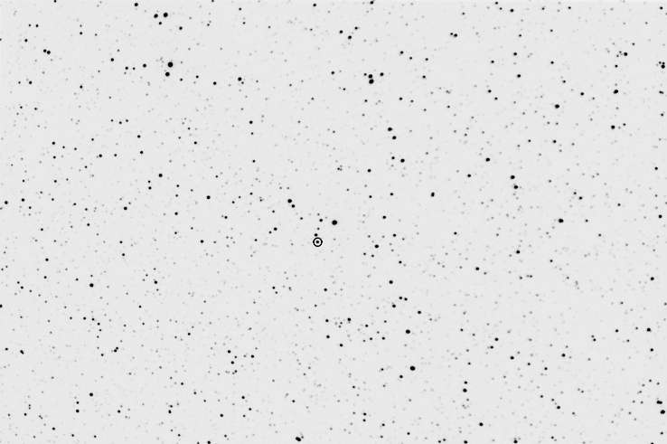
Figure 16. Wide angle field of view, 69 x 46 'arc,
with TrES-1 circled.
The following image shows which three stars I use as "reference
stars" (also called "comp stars") by the MaxIm DL Photometry Tool.
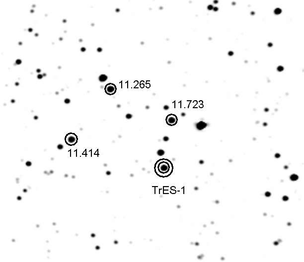
Figure 17. Zoomed and cropped version of previous
image, FOV = 14 x 12
'arc. TrES-1 is indicated by a double circle, and three reference stars
with their V-magnitudes are shown.
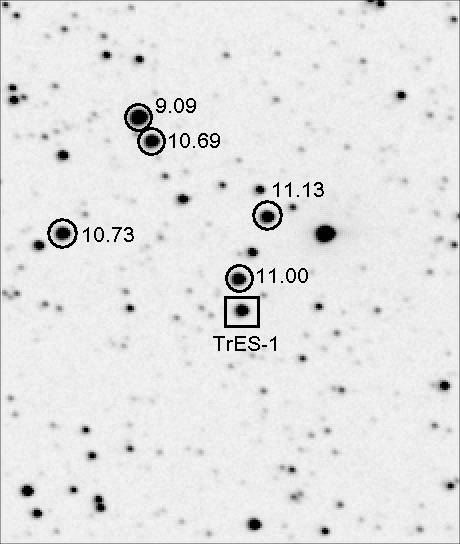
Figure 18. R-band reference star magnitudes. FOV =
10.8
x 12.7
'arc.
Links
for Text Data Files
To download the text data files of my transit observations click on
any of the following links, copy the displayed data to your Windows
clipboard, open Notepad, paste the contents of the Windows clipboard to
the blank Notepad document, save the Notepad document, and finally
import that document to an Excel (or whatever) spreadsheet. Each datum
represents ~150 seconds of total exposure time (for the last two
dates);
each datum (for the last two dates) is a median combine of 5 exposures,
each 30 seconds long
(which removes cosmic ray artifacts).
2004.10.08
2004.10.02
2004.09.23
Links to other relevant sites
TransitSearch
summary of TrES-1 transit light curves
My exoplanet
observing tutorial
Bruce's
AstroPhotos
Amateur Exoplanet Archive
Exoplanet Observing for Amateurs (book)
My e-mail address is b g a r y @ c i s - b r o a d ba a n d . c o m
____________________________________________________________________
This site opened: October 10,
2004. Last Update: November 22,
2007