This web page describes the procedure I currently use for conducting all-sky photometry.

I like introducing the concept of all-sky photometry with the above example. It captures the notion that the concepts involved are simple, and easily understood. However, it is misleading because to do all-sky photometry right there are many details that have to be managed carefully and systematically. A good starting point for illustrating subtle effects is what I'll refer to as the "generic photometry equation":

   Magnitude = Z - 2.5 × LOG₁₀ ( Flux / g ) - K' × AirMass + S × StarColor  + S2  × AirMass × StarColor                                                                               (1)

    where Z is a zero-shift constant, specific to each telescope system and filter (which should remain the same for many months),
    Flux is the star's flux (sum of counts associated with the star). It's called "Intensity" in MaxIm DL,
    g is exposure time ("g" is an engineering term meaning "gate time"),
    K' is zenith extinction (units of magnitude per air mass),
    S is "star color sensitivity." S is specific to each telescope system (and should remain the same for many months),
    StarColor can be defined using any two filter bands. B-V is in common use; I use 0.57 × (B-V) - 0.33,
    S2 is a second-order term that is usually ignored because it is only important for high air mass and extremely blue or red stars.

This general equation is true for all filter bands (even unfiltered), though there are different values for the constants for each filter. For example, the magnitude equation for V-band (omitting the last term in Eqn 1) is:

    V = Zv - 2.5 × LOG ( Flux / g ) - Kv' × AirMass + Sv × StarColor                                                                                                                                            (2)

Similar equations exist for bands B, Rc, Ic, g', r' etc. 

Notice that in a "generic photometry equation" for a specific filter there are two terms associated with a telescope system that should remain constant (provided there are no hardware configuration changes). This is illustrated for V-band:

    V = Zv - 2.5 × LOG ( Flux / g ) - Kv' × AirMass + Sv × StarColor                                                                                                                                           (3)

Zv and Sv are highlighted in green, and the task of "photometrically calibrating a telescope system" amounts to evaluating these two constants, as well as their counterparts for any other filter band of interest. Since extinction is different each night the K' terms have to be established each observing session; at least this is a common initial response to a review of the above equation.

I've chosen to define StarColor = 0.57 × (B-V) - 0.33 because it is zero for typical stars. This is an arbitrary choice but it is convenient for an iteration procedure I employ (described below).

NAIVE ALL-SKY PROCEDURE

When I began to perform all-sky photometry I endeavored to measure all the unknowns in Eqn (1) each all-sky observing session. I would do this for the 4-filter set B, V, Rc and Ic. This entailed observing standard star fields at many elevations and solving for Zj, Kj', Sj and S2j, for filters j = B, V, Rc and Ic. This permitted me to observe the target star at any elevation. Since I also solved for Kj' trends I could observe the target at any time of the night and minimize the effect of slow, monotonic extinction trends. This procedure involved lots of work; usually a full night of manual observations and several days of analysis.

It became apparent to me that the second-order term, S2×AirMass×StarColor, was always close to zero and its coefficient, S2, couldn't be established accurately enough to justify its use, so a few years ago I discontinued using this term. I also noticed that the star color sensitivity coefficient, Sj, didn't vary with observing date - provided the telescope configuration wasn't changed. I slowly adopted the habit of combining a night's Sj determination with an average of those from previous all-sky observing sessions.

Later I noticed that whenever my extinction coefficient was measured accurately I could count on the zero shift offsets, Zj, to be the same for many months. But when extinction wasn't measured accurately there was a relation between Zj and Kj', wherein a parameter relating the two coefficients was well-established but neither could be determined by itself. It was apparent that if the target and standard stars were at the same air mass the "degeneracy" of the Z-K' parameter pair wouldn't affect the results. But it was observationally difficult to observe all standard star fields at the same elevation.

These seveal learning experiences guided me to a variety of short-cut observing and analysis procedures. I'll now describe the next-to-last short-cut that I've used, or "partial all-sky" procedure.

PENULTIMATE ALL-SKY PROCEDURE

Since zenith extinction is usually different on each bserving date, and is time-consuming to measure, a commonly recommended strategy is to observe a set of standard stars and the target star when they are at the same air mass and at the same approximate time. The standard stars are used to evaluate the sum of the two terms Zj and Kj'×AirMass. This is equivalent to re-arranging the above equations to the following, for each filter band j:

    { Zj - Kj' × AirMass } = Mj + 2.5 × LOG ( Flux / g ) - Sj × StarColor                                                                                                                                      (4)

Let's call the bracketed term on the left Q for filter band j. Let's assume for the moment that Sj is known (based on many previous all-sky observing sessions; more on this below). Notice that all other items on the right side are known for standard stars (magnitude Mj and StarColor) or can be measured (Flux and exposure time, g). It is therefore possible to evaluate Qj using many standard stars.

    Qj  = average { Mj + 2.5 × LOG ( Flux / g ) - Sj × StarColor }  for many standard stars                                                                                                             (5)

The above Q for filter band j can be determined from the observation of a field of standard stars, and it is valid for one air mass value and one time of the night. Any target stars that are also observed at this air mass value and close in time can have their magnitude for filter band j evaluated using the following equation:

   Mj = Qj - 2.5 × LOG₁₀ ( Flux / g ) + Sj × StarColor                                                                                                                                                                    (6)

The parameter StarColor in the above equation is the target star's color. This, of course, is initially not known. My approach to this is to employ an iterative procedure after data for two bands is available, such as B and V. The iteration converges very fast (2 or 3 iterations), so this is not a problem.

The above procedure requires that the standard stars be observed at the same approximate air mass as the target star. If extinction trends are suspected then it is possible to observe standard star fields before and after the target star (at the same air mass), and interpolate Qj in time.

A method for quickly evaluating whether or not Sj has changed from the average of previously measured values is described in a section below.

I liked this procedure until I experimented with a variant of it. The next procedure, which I have now adopted as much better, illustrates an important shortcoming of the procedure just described: namely, the inability to identify the presence of cirrus clouds. 

ASSESSING SKY CONDITIONS FROM EXTINCTION PLOT

Sometimes I'm concerned about the possibility that even though a night begins with the appearance of being photometric (cloudless and calm) I could not rule out that during the all-sky observing session cirrus clouds could have drifted overhead. Regular cirrus is easily noted in the daytime, and in theory it could be monitored at night if there is moonlight. But there's an even greater threat to an all-sky observing session: subvisible cirrus. Even in daytime subvisible cirrus will usually escape attention. Subvisible cirrus is located just below the tropopause and defined as having an optical depth of < 0.05. This optical depths correspond to 50 mmag, which is important when trying to achieve an absolute photometry accuracy of half this amount (which is my goal). From an airplane flying near the tropopause these cirrus clouds are easy to detect visually (which I've done many times during my atmospheric science career, before retiring), but from the ground they are not usually noticeable - even when they have spatial structure. At night they are even less noticeable, especially from inside an observing control room. It is true that if these subvisible cirrus clouds lack spatial structure then they won't matter, but no cloud is devoid of spatial structure.

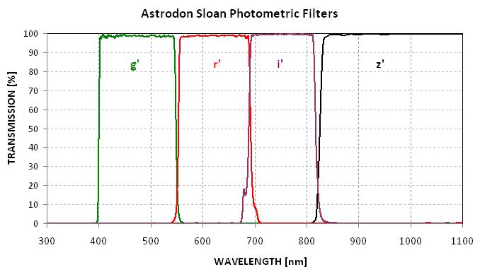
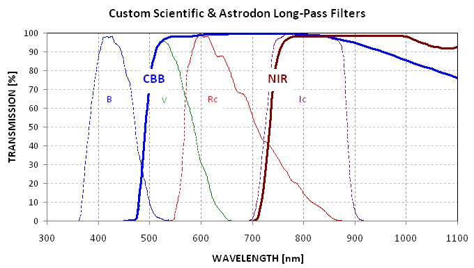
In response to this concern I have developed exerimented with another all-sky observing and analysis procedure designed to detect the presence of subvisible cirrus. It consists of an entire night's monitoring of a star field that has many standard stars within my FOV, with occasional breaks for observations of a target star. The large range of air mass that such an oibserving session provides allows for a determination of extinction to high accuracy for each band. I use a 10-position filter wheel, with the following filters: B, V, Rc, u', g', r', i', z', CBB and NIR. For each filter it's possible to fit an extinction curve and identify when clouds were present, if they were. Any filter is adequate for this purpose, so I prefer the one with a high SNR (such as V or Rc). Here's an example:


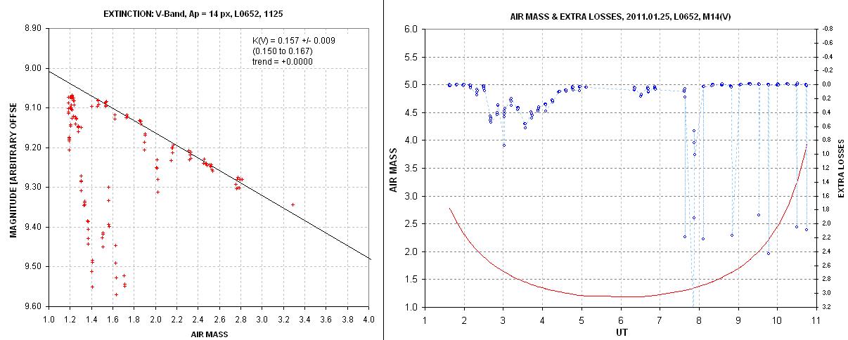
Figure 1. V-band extinction plot (left panel) and "residual losses" (right panel). Clouds render this observing session essentially useless, in spite of the evening's "photometric" beginning.

The left panels shows a fit to the envelope of bright readings. The night began looking photometric but after darkness episodes of cirrus clouds apparently drifted over my site. The extinction is well-established for clearings, and the right panel can be used to determine when these occurred (a plot with an expanded magnitude loss scale is used for this purpose). Even though this plot is based on observations of a standard star field (located at RA = 06:52) the extinction plot is made from flux readings of all stars in the field and the sum of fluxes is plotted. Any star field could be used for this purpose, since knowledge of star magnitudes is not needed for constructing these plots.

The target star was observed at ~ 5.5 UT, which the right panel shows was probably affected by cloud losses. Upon inspection of the extra losses plot I concluded that this observing session shouldn't be used for determining magnitudes for the target star. This is dramatic illustration of the fact that even when the sky looks perfect at dusk it would be foolish to assume that it will remain "photometric" during the rest of the night. I view this to be strong evidence for use of the "Simple All-Sky Procedure #2" instead of #1!

Five nights after the one just described another all-sky observing session was started at dusk during conditions that, again, appeared to be photometric. Here is the result of deriving V-band extinction for this observing session:


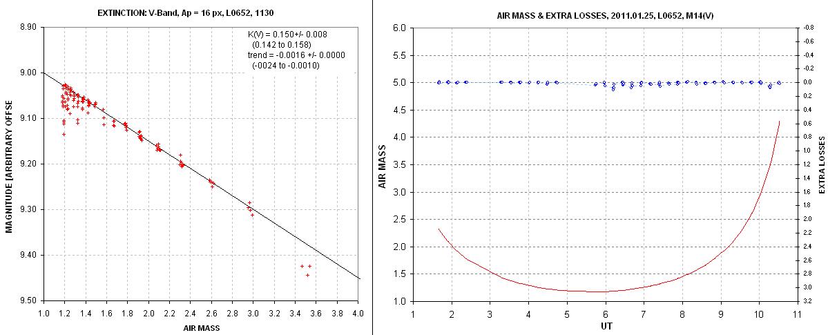
Figure 2. V-band extinction plot (left panel) and "residual losses" (right panel) for another date, 2011.01.30, when the observing session began during "photometric" skies. Subvisible cirrus appear to have been present at ~ 6.0 to 7.5 UT, and maybe 10.3 UT. At other times the sky appears to be photometric.

Again, the merits of relying upon "Simple All-Sky Procedure #2" instead of #1 are illustrated by the damatically better extinction and extra losses plot for Fig. 2 compared with Fig. 1; both nights began under photometric conditions but the first night deteriorated ~ 2 hours after sunset.

Here's an expanded magnitude scale version of the previous figure's right panel:


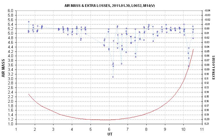
Figure 3. Expanded magnitude scale of "extra losses" plot for 2011.01.30, showing which observing cycles were well-behaved (low noise and no losses). Target stars were obseved at 3 UT, 5.3 UT and 11 UT.

The above figure shows that the first target star observation (~ 3 UT) was unaffected by clouds at the level of ~ 5 mmag. The second target star observations (~ 5.3 UT) may have been affected by losses of 10 or 20 mmag. These extra losses will render that target star's all-sky magnitude solution uncertain by at least 10 mmag, so it might not be wise to accept the magnitude solutions. However, since the observations with B and V filters are close together in time for each observing cycle it should be possible to rely upon the B-V star color solution. The third target star was observed after 10.6 UT, and since it was observed for 40 minutes (3 cycles) it might be possible to determine if any or all of its observations are cloud free based on the consistency of these observations.

Since the extinction plot makes use of the envelope of bright readings it is possible to obtain zenith extinction even for nights that are occasionally cloudy. A similar analysis of images for other filters allowed the following broadband extinction spectrum to be constructed. 

   
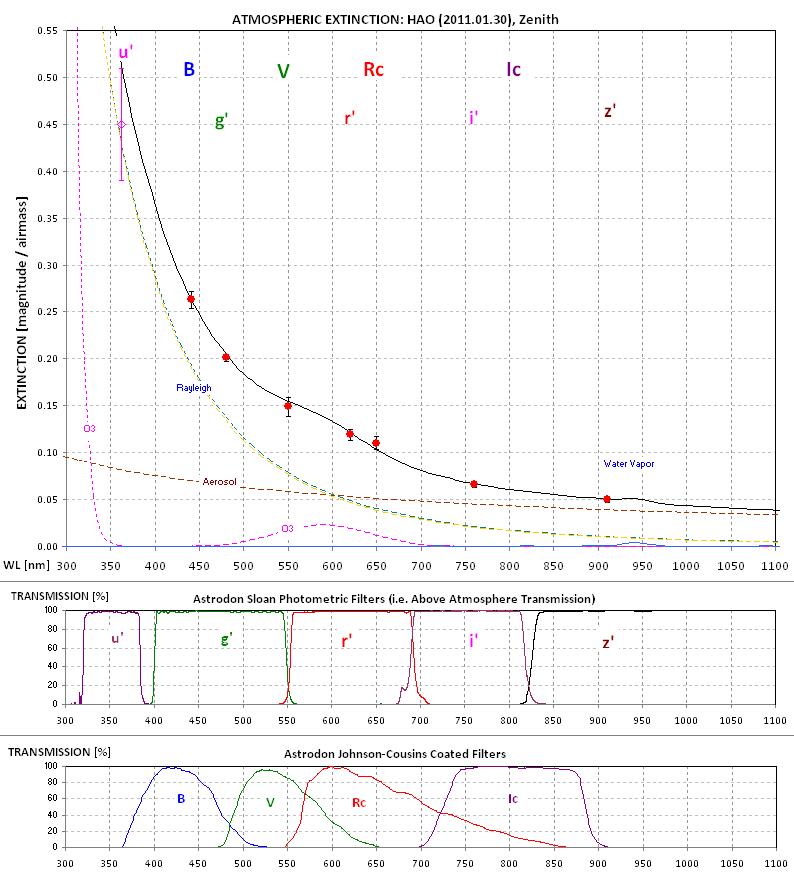
Figure 3. Broad-band spectrum of atmospheric extinction at zenith for the night 2011.01.30.  The 4 components of atmospheric extinction were adjusted to achieve a fit to the measurements (described in a section below). The Rayleigh component is essentially identical to that suggested by Hayes and Latham, 1975. (The u' extinction is left over from an earlier all-sky session, and it should be fairly constant for a specific observing site.)

The model fit extinction spectrum is statistically compatible with the measurements. The fact that the extinction measurements can be readily fit with this 4-component model suggests that the extinction measurements are accurate, and that a slightly better extinction value for each filter band can be obtained by reading the model fit (since it is influenced by all the measurements). This, in turn, means that it should be possible to derive an all-sky magnitude for target stars observed at air mass values not sampled by the standard star field(s), such as near zenith. This translates to flexibility in scheduling a night's observing session. For subsequent analyses it is possible to adopt extinction readings made of the model fit of all filters instead of the measurement for that filter. This may be advisable when extinction measurements are noisy, but on this occasion the extinction measurements are not noisy so I have adopted them instead of readings from the model fit.

SAFER ALL-SKY PROCEDURE (CURRENTLY-USED)

When plots of extra losses, such as Fig. 3 above, show that an observing session is found to be useable for determining target star magnitudes I proceed to process clear sky observing cycles of the standard star field for photometry measurement and analysis.

My observing sequence is gggrrrriiiiizzzzzRcRcRcVVVVVBBBBBBB, for exposures of 10 second each. This cycle requires 15 minutes to complete. For target stars I usually complete 3 cycles, but for the standard star field there will be ~ 30 cycles. A V-band image set is calibrated (bias, dark, flat), a hot pixel filter is applied to each image, and the images are aligned so that all stars are at the same pixel location. For example, when this is done for a cycle's V-band images there will be 5 calibrated and star-aligned images. Because some of the standard stars are faint I average this set of images (5 for V-band). (Note: median combining is totally inappropriate for all-sky photometry, only averaging is appropriate.) The averaged image is then measured by the photometry tool, which creates a CSV-file for later import to a spreadsheet.

When choosing a photometry aperture radius it is important to measure the fraction of flux captured by that aperture size. I do this by measuring a bright star in an uncrowded part of the image using a large aperture and one that is smaller by an amount that leads to a  magnitude change of ~ 20 mmag. Typically, this aperture radius is ~ 3 times FHWM. When the CSV-file produced by my image measuring program (MaxIm DL, v 5.12) is imported to a spreadsheet the magnitude readings are corrected for the lost flux fraction (e.g., the ~ 20 mmag correction).

When the above procedure is performed on several clear sky cycles for the standard star field, for one filter band, it is possible to begin the process of solving for the zero shift constant and star color sensitivity coefficient for that filter band. This is done by importing the CSV-files (created by MaxIm DL's photometry tool) to a template spreadsheet designed for this purpose. The spreadsheet uses JD and FOV coordinates to calculate air mass. Special parameters are calculated that have the feature that regardless of air mass when they are plotted their slopes correspond to the desired magnitude equation constants: Z, K' and S. I manaully search for fits by minimizing chi-square. The remainder of this section illustrates results of this analysis for the 2011.01.30 all-sky observing session.

The following plot illustrates a solution fit for determing S for Rc-band.

 
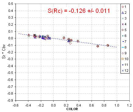
Figure 4. Plot of a parameter whose slope is S for Rc-band, based on 2011.01.30 observing session. The star field includes 26 calibrated stars in one FOV that were measured on multiple observing cycles (i.e., different air masses). The parameter plotted in the left panel takes into account air mass and corrects for it.

The data plotted in this figure can be at any air mass and the slope of this parameter with star color is the coefficient I refer to as S. Since this plot is for Rc-band images the slope corresponds to S(Rc). Notice the good correlation and small slope value. The small slope value means that my system's Rc-band response function resembles the standard Landolt telescope response function.

When S is derived this way it is compared with values from previous all-sky observing sessions to make sure it has not changed. The next figure shows S values determined from all-sky observing sessions during the past 8 months.


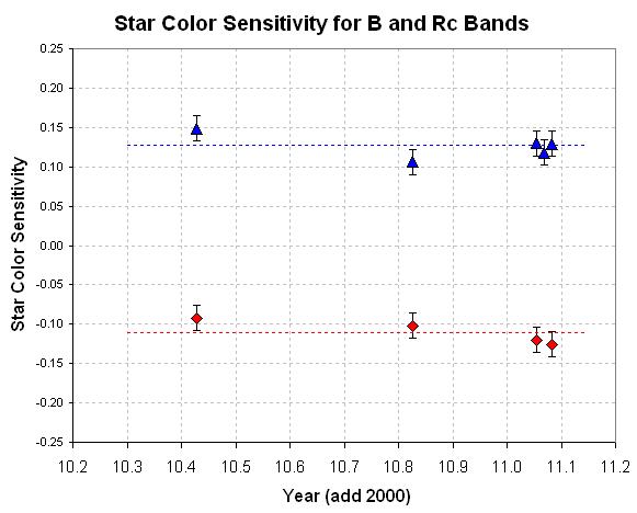
Figure 5.  Plot of Star Color Sensitivity for B and Rc bands, versus date (from 2010.06.04 to 2011.01.30), showing their stability during this 8-month period.

There is no evidence for a trend in either S(B) or S(Rc). It makes little difference whether subsequent analyses use the S value from the observing date or an average from a plot of past values when they are this well-behaved. Since the star color sensitivity coefficients appear to remain constant (provided I don't change the hardware configuration), it may be possible to simply adopt the average value from past all-sky sessions. However, I have decided to monitor these coefficients since I now have a calibrated star field with a sufficient number of stars within one FOV (26) that it is not difficult to verfiy that the coefficent value as not changes.

It is worth mentioning that even when an observing session can't be used for deriving target star magnitudes it is possible to derive star color sensitivity, S, because thin cirrus should not affect magnitude differences between stars of different color (since subvisible cirrus consists of ice particles large compare with visible wavelengths, and scattering is therefore Mie type). Even the zero-shift parameters, Z, for all filters can be determined by confining analysis to the clear images.

The next figure shows verification of the extinction value adopted from an earlier analysis (Fig. 2).


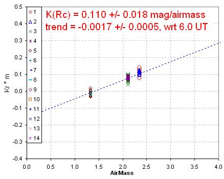
Figure 6.  Plot of a parameter that has a slope equal to zenith extinction. The extinction value, and its temporal trend, is set by the solution from another spreadsheet (see Fig. 2 for an example). 

I have the option of solving for zenith extinction (and its temporal trend) using slide bars in this spreadsheet. Although I used to solve for extinction this way I now use another spreadsheet designed for a long sequence of images for doing this more accurately (e.g., Fig. 2).

Once S and K' have been determined for a filter band it is possible to determine Z using a spreadsheet slide bar to minimize chi-square.

 
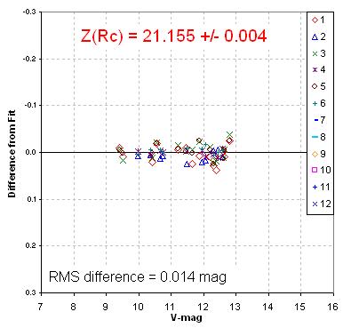
Figure 7.  Plot of differences between "true" Rc-band magnitudes and measurements using the "generic magnitude equation" with model fit values for S, K' and Z (for Rc-band).  

The RMS difference in this figure is 14 mmag, which is very good. Typically the RMS for this and other bands is ~ 20 to 25 mmag. I use an algorithm for identifying outlier measurements that is based on statistical theory and a criterion that for the number of measurements only the worst 25% of non-outlier measurements shall be rejected. This assures that un-modeled systematic effects (such as an imperfect flat field) won't influence the model fitting solution. Notice that scatter is greatest for the faintest stars.

At this point in the analysis of standard star images for one band it is possible to cmpletely specify the magnitude equation for the band. For the example just treated:

   Rc = 21.115 ± 0.005 - 2.5 × LOG₁₀ ( Rc Flux / g ) - (0.110 ± 0.007) × AirMass - (0.126 ± 0.011) × StarColor                                                                       (7)

The zero shift solution for this date is almost identical to the solution for 2011.01.20 (21.115 versus 21.158). This 3 mmag repeatability is a good indication that the hardware has not changed and the analysis is not seriously flawed for either observing date.

For the clear sky V-band image sets for this date the value for Z(V) was determined to be 21.073 ± 0.003, with a RMS scatter of 27 mmag (for 76 standard star flux readings).

The target star's color isn't known, so the V-band and B-band tentative solutions (starting with zero for star color) are iterated until convergence is attained. This leads to final values for V- and B-band magntiudes, which mean that StarColor for thetarget star has been determined, and can be used for the processing of the other bands.

The analysis procedure just described is possible because there is one star field with many calibrated stars within my FOV. The next section describes how I've increased the number of calibrated stars in a Landolt/Sloan star field from 19 to 26.

ENHANCED STANDARD STAR FIELD

The all-sky observing and analysis procedure just described can be performed best if just one standard star field has a large number of standard stars. If two or more standard star fields were needed to obtain a sufficent number of stars to establish a zero-shift parameter, and to verify the star color coefficient for each filter, then the observing session would be more complicated and more time would be spent acquiring the standard star fields - and this would require me to spend more time duing the night at the telescope controls (instead of sleeping). My telescope system has a FOV of 19.7 x 13.1 'arc, and an optimum placement of the FOV on the various Landolt/Sloan standard star fields produces ~ 6 Landolt standard stars and maybe one Sloan standard star, typically. The best Landolt/Sloan star field includes 19 Landolt stars and 4 Sloan stars, and it is located at 06:52:06 -00:22:30 (which I refer to as L0652). I have used the Landolt stars to calibrate 10 more nearby, bright stars, and so far they appear to be stable. Thus, this star field affords 26 stars for establishing zero-shift parameters, and star color coefficients, for the filter bands B and V.  For Rc-band there are 24 stars that I can use for this purpose. Eventually I may extend the 4 Sloan stars to some of the Landolt stars.

During winter nights L0652 rises shortly after dark and sets at about sunrise, so for this observing season it is possible to compare rising with setting data portions to determine temporal trends. For several months on either sideof L0652's optimum observing date (Jan 3) there will be sufficient air mass overlap to also determine temporal trends. During summer months, however, there is no comparable calibrated star field. One of my future projects is to enhance a Landolt/Sloan star field, such as L1745 or L2042, to create new standard stars within a single FOV.

FLAT FIELDING

I currently use either dusk or "dome flats." I've painted the zenith portion of the sliding door (when it's in the closed position) for this purpose. I use 4 lights (2 with blue coverage, and 2 with the standard yellow to red coverage). When taking dome flats I place a "double T-shirt" diffuser cover on the telescope aperture, and this reduces the effects of any non-uniformity of my illumination of the white spot atop the dome. Part of my motivation for performing flat field images using the dome was to avoid any effects that might exist when using dusk flats before the telescope had cooled. After achieving the capability of exposiing dome flats at any time during the night I demonstrated that focus setting doesn't matter; so now the dome flat capability is merely a convenience, and I do not claim that it offers a superior quality flat.

FILTER BANDS

____________________________________________________________________