DIFFERENTIAL PHOTOMETRY
ALTERNATIVE EQUATIONS
Bruce L. Gary, Hereford,
Arizona, USA
After deriving the "CCD Transformation Equations" a few years ago
I was convinced there should be a simpler way to accomplish the same
thing. My floundering with alternative procedures eventually paid off
and this web page describes simple procedures that are more accurate, more
intuitive and therefore less prone to book-keeping errors.
INTRODUCTION
If you're a "glutton for punishment"
then you are welcome to continue using the classical "CCD Transformation
Equations" for correcting raw mangitudes to "transformed" magnitudes.
I've derived these equations "from first principles" and have explained
how to use them at the following web page: http://reductionism.net.seanic.net/CCD_TE/cte.html.
If, however, you want to try using simpler methods, which I think are superior
in several ways, then this web page is another of my many attempts at offering
those alternatives. Two of them have the advantage of not requiring that
the telescope system be calibrated (using Landolt stars, or M 67). However,
my best alternative method assumes that this calibration has been made. Even
though this method and the classical one both require prior calibration of
your telescope system, my method is easier to use because it is more intuitive,
and it is less prone to book-keeping errors. Perhaps a more important advantage
of my method is that it does not assume that atmospheric extinction conditions
are similar to those when the telescope system was calibrated, which the classical
"CCD Transormation Equations" implicitly assume.
In spite of my preference for alternatives I recommend reading tutorials
using the classical method. I take this position in part because I am indebted
to them for motivating me to understand basic concepts. AAVSO has a good web
page describing a simplified version of the classical CCD Transformation Equations
that are suitable for amateur use: CCD
Observing Manual. That web site is an updated version of an early description
by Priscilla Benson, which used to be sent to new AAVSO members (link to PDF).
This was my introduction to CCD transformations 10 years ago, when I began
amateur astronomy, and I think this method is what most amateurs still use.
The organization of this web page can be summarized with the following
list of internal links:
1. Basic Photometry Equation
2. Calibrating the Telescope System
3. Differential Photometry - Method #1
- Recommended
4. Differential Photometry - Method #2
- Unrecommended
5. Differential Photometry - Method #3
- Unrecommended
6. All Sky Photometry for V, R and
r' Unfiltered - Novel Approach
7. Using r'-band Carlsberg
Meridian Survey for Determining V, R, I and r' From Any-Filtered Images
Section 1 describes the "basic photometry equation." It's an essential
starting point for understanding the several factors that determine a magnitude
measurement.
Section 2 describes calibration of a telescope system. I believe it
is essential that anyone doing differential photometry devote an entire night's
observing session to observations of Landolt star fields at least twice a
year. As an aside, I don't recommend that amateurs use M 67 for calibrating
unless their observing site has very good atmospheric seeing and the CCD image
scale is less than 1 "arc/pixel. M67 is fine for professionals, because they
have small FOVs and M 67 stars are close together, but this can be a problem
for amateurs with PSFs that spread one star's flux close to nearby ones.
I recommend using Landolt star fields at least twice a year for the purpose
of calibrating the telescope system, i.e., determining the telescope system's
star color sensitivities (Sb, Sv, Sr, Si and Sc, to use my terminology). Section
2 is a description of how to perform this calibration.
Section 3 illustrates my recommended procedure for performing differential
photometry. It assumes that the telescope system calibration is current. When
only two filter bands are of concern, V and R for example, the only parameters
that need to be "current" are Sv and Sr.
Sections 4 and 5 are optional reading. They describe a couple alternative
procedures that don't require a current telescope system calibration. They
are simpler to use than my preferred procedure, but I don't recommend them
unless you absolutely don't have time to perform the telescope calibration
observations (using Landolt stars or M67, etc) to derive good quality values
for the star color sensitivities. Two of these "short cut" methods are described
as Sections 4 and 5.
The following examples are
for just two filter bands, V and R. The reader is expected to "generalize"
the concepts illustrated using V and R to any two bands. These concepts can
therefore be generalized to more than 2 bands, i.e., to all four major bands,
BVRI. Even an unfiltered observation is a "band" and can be treated as such
using these concepts. Therefore, whereas I illustrate the concepts using "telescope
star color sensitivities" Sv and Sr, and their corresponding zero-shift parameters
Zv and Zr, these concepts are also valid for Sb, Si, Sc and Zb, Zi and Zc.
This web page looks long,
but understand that I have tried to explain things in enough detail that
extra thinking, between the lines, is not necessary. It should therefore be "fast reading."
1. BASIC PHOTOMETRY EQUATION
For any filter the following equation shows how key factors determine
measured star flux:
Mag = Z - 2.5 × LOG10
(Flux / g) - K' × AirMass + S × StarColor
(1)
where Z is a zero-shift constant, specific to
each telescope system and filter (which should remain the same for many
months),
Flux is the star's flux (sum of counts associated
with the star). It's called "Intensity" in MaxIm DL,
g is exposure time ("g" is an engineering term
meaning "gate time"),
K' is zenith extinction (units of magnitude),
S is "star color sensitivity." S is specific to
each telescope system (and should remain the same for amny months).
This is a general equation that is true for all filter bands (even unfiltered),
though there are different values for the constants for each filter. For
example,
V = Zv - 2.5 × LOG (Flux / g) - Kv' ×
AirMass + Sv × StarColor
(2)
R = Zr - 2.5 × LOG (Flux / g)
- Kr' × AirMass + Sr ×
StarColor
(3)
Similar equations exist for bands B and I (the rest of this web page uses
only V and R to illustrate concepts).
Note that some observers like to add the term SM * AirMass * StarColor,
where SM is a constant specific to each telescope system and filter band.
The value of SM is usually so small that I will ignore it in the following.
Note that I haven't defined StarColor. It can be defined using
any two filter bands, with B-V, V-R, V-I in common use. For this web page
I'll use:
StarColor, C = V-R-0.4
Why, you may ask, do I subtract 0.4 form V-R in defining C? By doing this
I've defined C in such a way that for typical stars have C ~ zero, and this
color term can be ignored if you don't know a star's color and don't mind
having errors of ~ 0.03 mmagnitude due to that assumption.
To illustrate eqns 2 & 3 using my 14-inch telescope:
V = 19.81 - 2.5 × LOG (Fv/g)
- 0.16 × AirMass - 0.07 ×
C
(4)
R = 19.95 - 2.5 × LOG
(Fr/g) - 0.11 × AirMass - 0.10 ×
C
(5)
where Kv' ~ 0.16 [mag/airmass] and Kr' ~ 0.11 [mag/airmass] typically,
and Fv and Fr are fluxes from V-band and R-band images
Similar equations exist for B, I and C (clear). I find these equations
handy for quickly calculating magnitudes when I don't want to bother consulting
a star catalog for setting MaxIm DL's magnitude scaling. To illustrate
how easy this method is, consider the case where a V-band image is made
at m = 1.5 with an exposure time g = 60 seconds and a star is measured to
have F = 10,000 counts. Let's set C = 0, and solve for V = 19.81 - 2.5
* LOG (10,000/60) - 0.11 * 1.5, or V = 14.09. I've checked stability of
the constants Z, K' and S for all bands and indeed they are pretty constant
for many months, provided I don't change optical configuration (or let
the corrector plate collect dust). I think this equation alone can produce
results with an uncertainty of ~0.06 magnitude.
Differential photometry is more accurate, able to achieve SE ~ 0.025 to
0.030 magnitude, for example. As a minimum, this can be done using images
with two filters of a star field that includes one star that is calibrated
(has known magnitudes for the filter bands in question). Using the calibration
star it is possible to determine magnitudes for all other stars in the
image. If only one star in the image is calibrated, however, results will
be marginal and it will be necessary to employ Differential Photometry Method
#1, which in turn assumes that the telescope system has been calibrated using
Landolt stars. If, on the other hand, the target star image set includes in
the FOV several calibrated stars ("comp" stars), it is possible to perform
differential photometry of the target star(s) without having performed Landolt
star calibrations of the telescope system. For this case the several calibrated
stars can serve to establish approximate values for star color senitivities
and zero shifts. Accuracy won't be as good, but until the Landolt star calibration
is performed it's the only alternative.
2. CALIBRATING A TELESCOPE SYSTEM
USING LANDOLT STARS
Typically more than a half dozen stars are required to obtain a useable
version of the telecope system's "star color sensitivity parameters" Sv
and Sr (or Sb for B-band, Si for I-band and Sc for clear). I'll refer to
these as S-parameters; they're the only parameters that need to be calibrated
ahead of time in order to use this differential photometry method. I recommend
frequent ( at least twice yearly) calibration of the S-parameters.
S-parameters can be determined by observing a group of calibrated stars
that fit within a FOV, for which the many Landolt star fields are ideal. The
calibrated star fluxes are measured and used to produce instrumental magnitudes.
Differences between true and instrumental magnitudes for a filter band are
plotted, and the slope to that plot corresponds to the S-parameter for that
filter. This is illustrated by the next two screen captures of a spreadsheet
that performs these calculations. Real observations of two Landolt star fields
were used (L0652, for example, is my terminology for Landolt star field at
RA = 06:52).
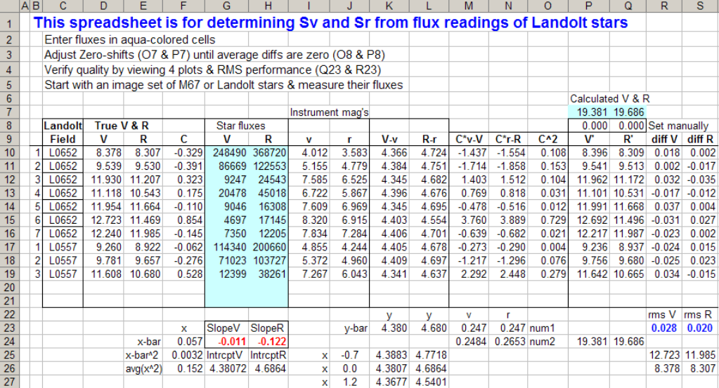
Figure 1. Spreadsheet
that calculates Sv and Sr (or Sb or Si or Sc) from a set of calibrated stars.
For this example Sv = -0.011 and Sr = -0.122.
The RMS difference detween true V & R magnitudes and those calculated
using these Sv & Sr values is 0.028 and 0.020 magnitude.
Sv is calculated by LS fitting a slope to the plot "V-v versus C." Similarly,
Sr is the slope of "R-r versus C." This is illustrated by the following plots.
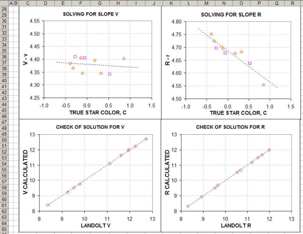
Figure 2. Upper
pair of plots show how fitted slopes to V-v and R-r versus star color C are
used to determine Sv and Sr.
Bottom plots show that V and R calculated from magnitude equations that
use Sv and Sr produce good quality results.
The spreadsheet that performs
these calculations is at: DP-Gary.zip (also includes
Method #1, below).
3. DIFFERENTIAL PHOTOMETRY -
METHOD #1 - MY RECOMMENDATION
When the telescope system has been calibrated, as described in the previous
section, we have information about S-parameters. For this example we know
Sv and Sr. This is all we ned for performing differential photometry using
my "recommended" Method #1.
The following screen capture is from the same spreadsheet that was used
to solve for Sv and Sr, used for illustration in the previous section. It
shows flux reading from another landolt star field (on the same night used
to solve for S-parameters, but Landolt stars at different air mass). The values
for Sv and Sr are entered in cells G76 and J76. Landfolt star V and R magnitudes
are entered, as are measurements of star fluxes. The spreadsheet calculates
zero shifts that can be used for the same image set (but not any other image
sets).
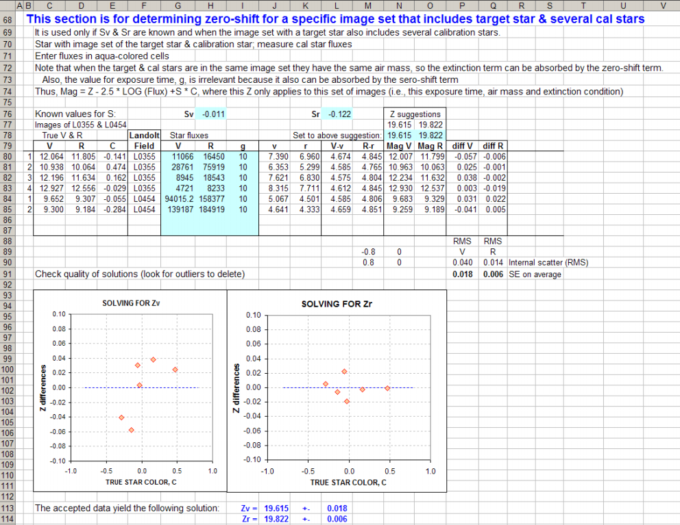
Figure 3. Zero shift
values for V- and R-bands are determined from a set of stars from two Landolt star fields.
The zero shifts Zv and Zr are obtained by adjusting the values in cells
L78 and M78 to agree with the suggested values (cells L77 and M77). When this
is done we have agreement between instrument magnitudes and the Landolt V
and R magnitudes. Keep in mind that instrument magnitudes are defined in this
spreadsheet according to the general equation: Mag = Z - 2.5 * LOG (Flux/10)
+ S * C. Extinction is irrelevant here because all stars are from one image
set that was made at one air mass. Other stars, such as target stars, will
be at the same air mass and will experience the same extinction. That's why
we can ignore the extinction term in the magnitude equation.
For the next step we simply enter measured fluxes for target stars with
the beginning assumption that their star color is zero (i.e, "typical"). This
is illustrated in the next screen capture of a lower section of the same
spreadsheet.
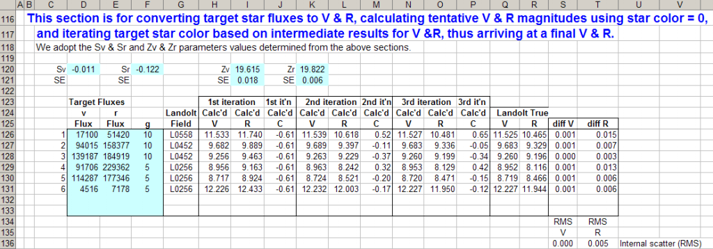
Figure 4. Three
steo iteration solving for target star V, R (and therefore C). RMS accuracy
for V- and R-bands is < 0.001 & 0.005 magnitude.
The stars chosen to be target stars in the above spreadsheet section are
from different Landolst star fields than were used for deriving S-parameters
and Z-parameters, and they are at different air masses. In spite of these
differences the iteration achieves acceptable results for RMS differences
with the true, Landolt magnitudes.
If you want to try using the spreadsheet that produced these results it
can be dowloaded from: DP-Gary.zip.
4. DIFFERENTIAL PHOTOMETRY METHOD
#2 - Not Recommended Unless Desperate
Differential Photometry Method #1 refers to the case of knowing ahead
of time the star color sensitivities for the filter bands used, e.g., Sv
and Sr. Differential Photometry Method #2 is for the case of not
knowing any of the star color sensitivities ahead of time, but having
several calibrated stars in the FOV, since star color sensitivities are
determined during the course of solving for the unknown star magnitudes.
Here's the procedure I recommend for Differential Photomtery Method
#1 (it is derived from the "basic photometry equation" at another web
page link):
1) Measure "instrumental magnitudes" for the target
& calibration star in images made
with V-band and R-band filters. Call
them vt, vc and rt, rc.
2) Calculate "colors" for calibration and target stars:
Cc = Rc - Vc - 0.4
Ct = { (Vc - Rc) ×
( 1 + Sr - Sv) + (vt - rt) - (vc - rc) } / {
1 + Sr - Sv } - 0.4
(6)
3) Calculate the target star's V-mag and R-mag:
Vt = Vc + (vt-vc) +
Sv × (Ct - Cc)
(7)
Rt = Rc + (rt-rc) +
Sr × (Ct - Cc)
(8)
|
where the following abbreviations have been used:
Vc = known V-mag for calibration star,
Rc = known R-mag for calibration star,
Sv = V-band star color sensitivity (slope of plot: V-mag error
versus star color C, for several calibrated stars), explained more elsewhere,
Sr = R-band star color sensitivity (slope of plot: R-mag
error versus star color C, for several calibrated stars), explained more
elsewhere,
C = star color, defined to be V - R - 0.4,
Ct = star color of target star,
Cc = star color of calibration star,
Vt = V-mag of target star,
Rt = R-mag of target star,
vi = instrumental magnitude of star "i" = 2.5 ×
LOG10 (Fi / g) + zero-shift
constant (that doesn't matter),
Fi = flux of star i,
g = exposure time
Note that leading upper-case letters are "true" magnitudes, e.g., Vt
is true V-mag for target, Vc is true V-mag for calibration star.
Leading lower-case letters are "measured instrumental magnitudes", e.g.,
vt is measured V-band instrumental magnitude of target (can have any
zero-shift). Second letter for magnitude sybmol refers to either "target star"
or "calibration star." Star color sensitivity for V-band is Sv, and
star color sensitivity for R-band is Sr. Both are assumed to be known
prior to this analysis.
An example of using these equations is given at Example1.
If there are more than one calibrated star in the FOV the above process
can be repeated for each star, and the results can be averaged.
5. DIFFERENTIAL PHOTOMETRY METHOD
#3 - Not Recommended Unless Desperate
This method is possible when there are several calibrated stars
in the same star field containing the target star. The method is required
when Sv and Sr have not been determined from an observing
session of M67 or a Landolt star field. The classical "CCD Transformation
Equations" are designed for this situation, and the procedure described
in this section achieves a comparable result.However, this is not my favorite
method because "star color senitivites" for the telescope system can never
be established as accurately as can be achieved by a special observing session
of M 67 or Landolt stars.
[This section is under development]
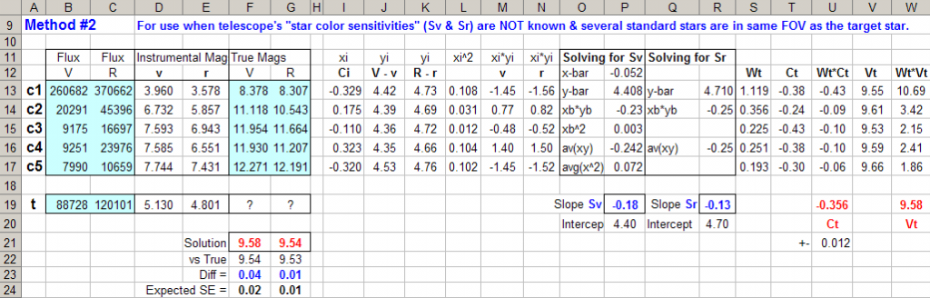
Figure 5.
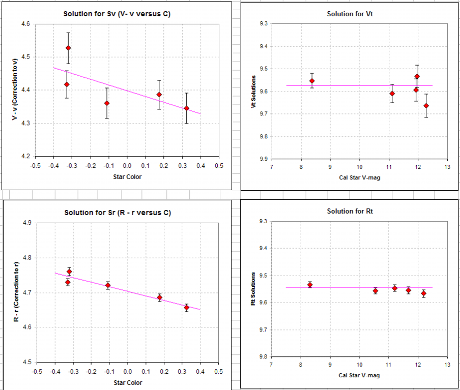
Figure 6.

6. ALL SKY PHOTOMETRY FOR
V, R and r' USING UNFILTERED IMAGES - A NOVEL APPROACH
Few people realize that it's possible to derive V, R and r' magnitudes
of an target star from unfiltered observations anywhere in the sky. The key
concept that makes this possible is that J and K magnitudes, which are present
for almost all stars between V-mag ~ 9 and 17.5, and star color, C, can be
derived from J-K with pretty good accuracy. Knowing C allows unfiltered star
fluxes to be converted to magnitudes for any band if the telescope system
has been calibrated for this purpose. This section will illustrate the procedure.
My Celestron 11-inch telescope is currently configured without a color
filter wheel, and I intend to continue with using this configuration. Sometimes,
however, I want to measure a star's V- or R-band magnitude using unfiltered
images, so I developed a procedure that allows this. I will illustrate this
using images taken of four Landolt star fields, with a total of 28 Landolt
stars. Here is the set of Simplified Magnitude Equations that are used for
this purpose:
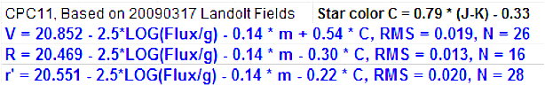
Figure 7. Simplified Magnitude Equations for use with unfiltered
images with my 11-inch telescope. C is derived from J and K magnitudes.
For these equations C = 0.79 * (J-K) - 0.33, which produces a value siliar
to C = V - R - 0.4 (with RMS difference on C of 0.03). The JK-based C is
illustrated by the following scatter diagram of 16 comparisons:
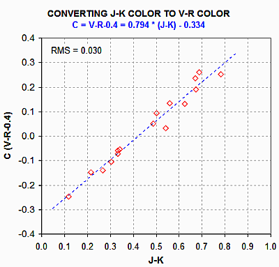
Figure 8. Converting J-K to my standard star color C = V-R - 0.4.
The equations in Fig. 7 are derived from the slope of plots of one observed
parameter versus another for a set of stars having different colors. I won't
go into detail about this because it is all handled by worksheets in the
above-mentioned spreadsheet DP-Gary.xls. Here's a screen shot for V-band
that shows the two most important plots (on left):
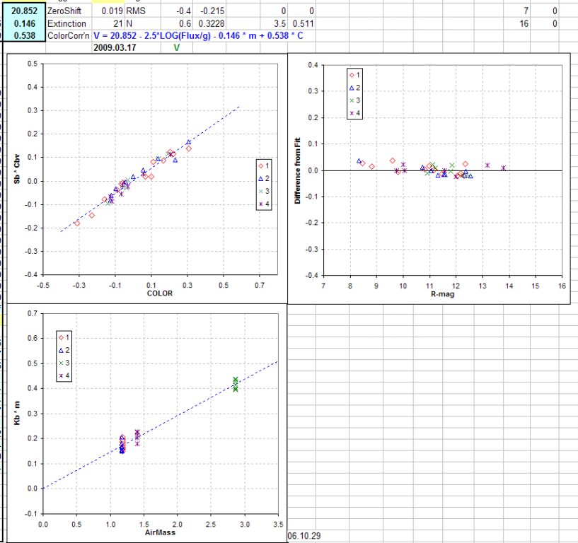
Figure 9. The slope of the upper-left plot is +0.54, which is the
color sensitivity parameter for V-band. The lower-left plot is merely a way
to estimate zenith extinction, which is needed for determining the zero-shift
parameter. The upper-right panel shows differences of fitted V-band magnitudes
using the SME for V-band and the true V-band (Landolt) magnitudes. Four Landolt
star fields with a total of 21 stars were observed. The RMS difference with
true (Landolt) magnitudes is 0.019 magnitude. Star color was derived using
C = 0.79 * (J-K) - 0.33.
Similar plots for R-band and r'-band allow evaluation of the rest of the
parameters in Fig. 7.
For asteroids, which do not have J and K magnitudes, it may be assumed
that C = 0.00 ± 0.08. The SE of 0.08 translates to SE for V-band of
0.04 magnmitude, and smaller uncertainties for R- and r'-band.
7. USING r'-BAND
CARLSBERG MERIDIAN SURVEY MAGNITUDES TO DERIVE V, R, I and r' USING ANY-FILTERED
IMAGES
Related Web Page Links
AAVSO photometry manual: http://www.aavso.org/observing/programs/ccd/manual/4.shtml#2
Lou Cohen's 2003 tutorial: http://www.aavso.org/observing/programs/ccd/ccdcoeff.pdf
Priscilla Benson's (1990's) CCD transformation equations
tutorial: http://www.aavso.org/observing/programs/ccd/benson.pdf
Bruce Gary's
All-Sky Photometry for Dummies: http://brucegary.net/dummies/x.htm
Bruce Gary's All-Sky Photometry
for Smarties - v1.0: http://brucegary.net/photometry/x.htm
Bruce Gary's All-Sky Photometry for
Smarties - v2.0: http://brucegary.net/ASX/x.htm
Return to nominal calling web page: link
____________________________________________________________________
WebMaster: Bruce
L. Gary.
Nothing on this
web page is copyrighted. This site opened: 2009.03.10. Last Update: 2009.03.25