Image Subtraction Tutorial
Bruce L. Gary; 2005.10.09
Abstract
This web page describes an "image subtraction" procedure for
determinatining the light curve of very faint asteroids in crowded star
fields. The example light curve for a 20.4 magnitude asteroid uses
amateur hardware and an image analysis software commonly used by amateurs (MaxIm DL). Professionals typically use PSF-fitting
programs to extract faint objects from crowded star fields, but this
requires the use of long-learning-curve programs, such as IRAF, which
cannot run on Windows-based computers. Image subtraction may in fact be
superior to PSF-fitting for moving asteroids since it reduces background stars to approximately 1% of their original level and
leaves the asteroid's image unaffected at the 100% level. Image
subtraction procedures are tedious, but hopefully parts of it
can be automated and someday become commercially
available.
Links Internal to this Web Page
Introduction
Observations on 2005.09.26
Image Subtraction Procedure
All-Sky Calibration
3-image Example Using a Smaller Telescope
Introduction
This observing project is meant to show that amateurs are
capable of measuring the light curve of asteroids fainter than
magnitude 20 using an image subtraction procedure and a Windows-based
astronomical image processing program (MaxIm DL). Images from a 3-hour
observing session on 2005.09.26 UT are used to illustrate the
procedure. Observations were made 25 days earlier with the same
telescope but it is not necessary to describe them for the purposes of
this tutorial.
Observations of 2005.09.26
A 3-hour observing session was conducted on 2005.09.26 UT
with the Junk Bond Observatory fork-mounted 32-inch Ritchey-Chretien
telescope system (built by Optical Guidance System). The telescope is
housed in a computer-controlled 16.5-foot dome. The CCD camera is a
SBIG model STL-6303E. It is a large format CCD (27.7 x 18.5 mm main
chip) that employs a KAF-6303E main chip having a 3072 x 2048 pixel
layout (9 micron square pixels size). All components are
computer-controlled
except the focusing, which is reliably constant due to the telescope's
low-to-zero expansion invar cage. All exposures were 2-minutes and were
unguided.
Asteroid "46053
Davidpatterson" is a main belt asteroid with an ephemeris H = 16.2. At
the time of these observations the asteroid was predicted to have a
V-magnitude of 20.12. It's location was ~22 degrees from the galactic
center and the star field was more crowded than
ususal. Aperture photometry, and even PSF-fitting, are difficult to use
in crowded star fields. The combination of a faint asteroid in a
crowded star field is an ideal situation for using image subtraction.
Image Subtraction Procedure
Master flats and darks were used to calibrate 86 raw images of the
asteroid region. During the 3-hour observing session the asteroid’s
apparent motion
was many times the FWHM width of star images. This allowed for the
creation
of a “reference image” using several images when the asteroid was far
from its
location in a “signal image.” Since 4 to 8 images were used to create a
reference
image its subtraction from a signal image led to a “subtracted image”
having a
noise level only slightly greater than the noise level of the original signal image. Before subtraction the
FWHM of
the two images were checked for a match, and if they differed the
reference
image was either sharpened or smoothed to achieve a match. The flux
(i.e,
intensity) of a specific star was checked for equality, and the
reference image
was rescaled (during the subtraction process) to achieve a match.
Here's an example of image subtraction (for a set of 4 images).
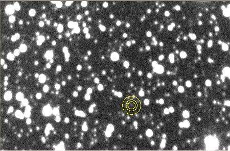
Figure 1. Before image subtraction. Note the barely visible
asteroid (CV = 20.0) at the center of the photometry aperture circles. The stars to
the upper-right of the asteroid have V-magnitudes of 16.2. FOV = 7.2 x 4.7 'arc, north up, east left.
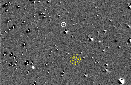
Figure 2. After
image subtraction. Top circle is the "offset alignment dot." The
3-circle photometry pattern is cenetered on the asteroid, which is
easily visible.
These two images give a preview of what can be expected when using
image subtraction. Many small steps are required to achieve these
results.
The most tedious part of this process is image
alignment.
For the observations reported here the asteroid moved a significant
fraction of
a FWHM distance between images. This meant that images could not be
stacked (median combined) using the star field. This, and other
considerations,
led to a sequence of manipulations that are described here using MaxIm
DL (after calibration and cropping to the same approximate
FOV):
1)
Median combine (MC) 4 images using star
alignment.
2)
Select a bright (unsaturated) “offset reference star”
for later use in all images; note its FWHM and intensity. Calculate an air mass value for this 4-image group.
3)
Repeat steps 1 and 2 for all images.
These sets of images (each a 4-image median combine) are available for
use as "subtraction reference images."
4)
Start with the first group of 4 “signal images”
and choose a "subtraction reference image" (from step 3) that was taken > 1 hour from the time
of the signal images. Select an image that has a FWHM similar to those for the 4 signal images.
5)
Either sharpen or smooth the reference image so
that its FWHM is similar to the 4 signal image FWHMs.
6)
For each signal image note the UT start time and
the offset reference star’s x,y coordinates and intensity. Use a spreadsheet to
calculate the expected motion of the asteroid since some arbitrarily chosen
start time (such as the first image of the entire series).
7)
Pixel edit an “alignment dot” at a location that
differs from that of the “offset reference star” by the calculated asteroid’s
expected motion for that image (plus an x,y offset that is constant for the
observing session).
8)
For each signal image (now having an alignment
dot) use the alignment command; select the signal image first, then the
reference image (to assure that the x,y coordinates of the alignment dot do not
change), and use automatic star alignment.
9)
Perform an image subtraction (Process/Pixel
Edit); select the signal image first, then the reference image (for the reason given
above). Keep the signal image at 100% and adjust the reference image to whatever
% will bring its intensity scale into match with the signal image.
10)
Repeat steps 7 – 9 for the other 3 signal images.
You should now have 4 “subtracted signal images.”
11)
MC the 4 “subtracted signal images”
using the
alignment dot to produce a “MC'd group-of-4 signal subtracted image.” Since
it is a MC of 4 (signal subtracted) images it should be free of cosmic
ray defects
and hot or cold pixel defects associated with imperfect calibration.
12)
Calculate the asteroid’s expected
x,y location,
based on the RA/Dec coordinate differences between the “offset
reference star”
and the asteroid (from an ephemeris) at the arbitrarily chosen start
time (see Step 6), and adjusting for the constant x,y offset used in
Step 7.
13)
Measure the flux (called “intensity”
in MaxIm DL)
of the location where the asteroid is supposed to be located. (Notice
that the asteroid doesn't have to be visible in any of the images for
this procedure to work.)
14)
Determine the asteroid’s magnitude using the
measured flux and air mass (using eqn. 1, below).
15)
Repeat steps 4 to 14 so that all images are
treated as signal images in groups of 4.
Converting flux to magnitude (Step 14) can be done in
several ways. My preferred procedure is to enter flux, S, into a spreadsheet
cell that uses the following "simple magniutde equation":
CV = Zcv – 2.5 * LOG
(S / g ) – Kcv * m + Scv * C
(1)
Where CV is V-magnitude equivalent using a clear filter, Zcv
is a zero offset determined for a night’s observing session from observations
of a field of calibrated stars (Landolt, Henden, Skiff, etc), S is star flux
(referred to as “intensity” in MaxIm DL), g is exposure time [seconds], Kcv is
zenith extinction for typical stars [magnitude/air mass], m is air mass, Scv is
your telescope system’s star color sensitivity (determined a few times per year
and spot-checked using Landolt stars), and C is star color, defined as (V-Rc) -
0.31 (C is defined so that a typical star has C ~ 0; a typical asteroid has C ~
+0.09). (For an extensive discussion o this unusual procedure for converting flux to magnitude go to http://brucegary.net/photometry/x.htm).
Aperture size is an important consideration when
working with faint objects and when the star field is crowded. For the
case of a Gaussian PSF the signal aperture provides an optimum SNR when
its radius is set to 3/4 of the FWHM. The SNR payoffs for choosing a
small signal aperture can be quite large, such as a factor of two
(corresponding to a factor of 4 in observing time). Other
considerations argue for a sligfhtly larger signal aperture circle
(differences in PSF in the same image, etc). For faint objects I
usually adopt an aperture radius about twice this optimum value (i.e.,
radius ~1.5 times FWHM). If the star field is crowded I prefer a
slightly smaller aperture. For these observations I chose 1.2 times
FWHM. There's a downside to using a small signal aperture; less than
100% of the object's flux is "captured." For these observations
with a signal aperture radius of ~1.2 * FWHM the "recovery fraction"
was ~90%. In order to convert measured flux to a magnitude using the
above "simple magnitude equation" it is necessary to correct flux
measured with a small aperture to expected flux with a large aperture.
This correction is necessary because the constants and coefficients in
the above equation are based on observataions of standard stars
(Landolt, Henden, Skiff catalog) using a large signal aperture. Why,
you may ask, are the standard stars measured using a large aperture?
Because only when close to 100% of their star image is "captured" can
the constants and coefficients be counted on to remain the same for
many observing situations (with different seeing conditions, different
focus settings, etc). In the above equation the flux term, S, is for a large signal aperture. When the asteroid is measured using a small signal aperture, for which the recovery factor f is known, the measured flux S' must be converted to its large aperture equivalent using S = S' / f, where f is the ratio of small aperture flux to large aperture flux (f < 1). The simple magnitude equation must therefore be amended to the following:
CV = Zcv – 2.5 * LOG
( (S'/f) / g ) – Kcv * m + Scv * C
(2)
The recovery fraction f depends upon FWHM, and since seeing changes during an observing session f
must be measured whenever FWHM changes. I chose small aperture
photometry dimensions of 6/4/7, meaning that the signal aperture radius
was 6 pixels, the gap annulus width was 4 pixels and the sky background
annulus width was 7 pixels. I will refer to the recovery fraction for
this photometry setting as f647. Step 2 and 14 should be amended to the following:
2)
Select a bright (unsaturated) “offset reference star”
for later use in all images; note its FWHM and intensity using the small aperture (6/4/7). Determine f647 using the bright offset reference star. Calculate air mass using a planetarium program (such as TheSky 6).
14)
Determine the asteroid’s magnitude using the
measured flux S' (using the small aperture photometry settings) and the recovery fraction f647
for that 4-image group. Employ pixel edit as necessary to remove
residual "star ghost artifacts" that are within the sky background
annulus.
When the asteroid had rotated to its faintest
phase it was usually not "visible" in the subtracted signal images.
Even the "MC'd group-of-4 signal subtracted images” often did not show
the
asteroid. Nevertheless, when the photometry aperture pattern was placed
at the predicted x,y location of the asteroid there was always a useful
flux with SNR > 5. Because of these low SNR values I resorted to a
parallel analysis by averaging pairs of “MC'd group-of-4 signal
subtracted images.” In the following graph the asteroid magnitudes
based on
“MC'd group-of-4 signal subtracted images” are shown with small green
triangles and the average of two of these images (total of 8 subtracted
images) are shown with red diamonds.
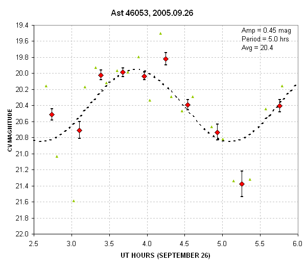
Figure 3. Light curve for 2005.09.26. Each green diamond is
based on 4 images (each having an exposure of 2-minutes). The red
diamonds are based on 8 images. The error bars are stochastic SE and do not include estimated systemtic uncertainties.
The average
brightness of 20.4 is ~0.3 magnitude fainter than expected based on the
ephemeris but is ~0.1 magnitude brighter than expected based on
2005.09.01
observations. The amplitude is also the same as 25 days earlier,
corresponding to a 0.90 magnitude peak-to-peak variation. The period is
also approximately the same.
I should comment about the SE error bars and their apparent Bayesian
incompatibility with the model fit. It is extremely unlikely that the
error bars are correct since there are many data points that depart
from the model by several SEs. The plotted SE bars are stochastic,
based solely upon SNR - specifically, SE = 1.1 / SNR. Systematic
uncertainties are undoubtedly present but they are very difficult or
impossible to evaluate prior to comparing the data to a reasonable
model. There are two cattegories of systematic SE: those that are
shared by all data, such as a photometric calibration error, and those
that can change during the observing session. This latter category is
obviously present as evidenced by the large differences between points
that are spaced closer in time than any light curve variation could
accomodate; the first category is probably present but it can't be
proven from anything evident in this data set. The "varying systematic
error" must be approximately 0.15 magnitude since this amount of error
would have to be orthogonally added to the stochastic SE in order for
the total SE to be compatible with the above plot. This 0.15 varying
systematic error, or ~15%, could easily be produced by an incomplete
star field subtraction. Typically, the star field subtraction is only
99% effective, leaving a residual ~1% feature in the subtracted image.
If a nearby star is 100 times brighter than the asteroid then the
residual feature would have the same amplitude as the asteroid. This
residual star feature could be within the signal aperture or in the sky
background annulus. In one case the apparent asteroid brightness would
be increased, while in the other case it would be decreased (assuming the residual artifact had a positive flux). The
amplitude of the increases would be larger than the amplitude of the
decreases, but there should be fewer increases than decreases since the
pixel area for the signal aperture is smaller than that for the sky
background annulus. Another predicted behavior for these residual
background features is that they should become important as the
asteroid becomes less bright. At some faint level the signature of
residual background stars should become the dominant component for all
measurements. The level where this happens will depend upon how many
background stars there are and how variable the seeing was. These observations were made close to the galactic
center (~22 degrees). Therefore the star density was greater than for a typical region of the
sky. Presumably, it should be possible to observe asteroids fainter
than this one (CV= 20.4) for determining light curves provided they are
at greater galactic latitudes.
Just for fun, I'm including an animation of the same
asteroid obtained when it was brighter on 2005.09.01, showing its
northwestward motion.
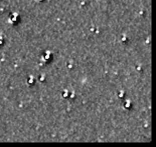
Figure 4. Animation of asteroid motion during the 2.7-hour 2005.09.01 observing session.
Photometric Calibration of Asteroid Star Field
The photometric calibration procedure for 2005.09.26 was quite different from the one for 2005.09.01.
The earlier observing session included BVRC observations of M27 (for
the purpose of monitoring the brightness of a recent cataclysmic
variable on the western edge of M27), and there were 7 bright stars
near the variable star that had been calibrated by Arne Henden. These
were used to establish a Zcv solution, and to check that Scv was the
same as determined using Landolt stars months earlier. An air mass
difference between M27 and the asteroid meant that the zenith
extinction coefficient Kcv had to be relied upon to establish a
calibration of stars near the asteroid.
The 2005.09.26 observing session did not include any all-sky
observations. Instead, a 14-inch Celestron was used on
2005.09.29 to calibrate stars near the asteroid's 2005.09.26 location.
Observations were made of 14 stars in the Skiff catalog with B and
V magnitudes that were located a mere 1/4 degree to the east of the
2005.09.26 asteroid location. The close proximity of the Skiff stars
and the asteroid location made it unecessary to refine the
zenith extinction value for transferring Skiff brightnesses to the
stars near the asteroid field. The 14-inch Celestron's telescope system
photometry constants had values similar to those on previous occasions
when Landolt regions were observed, and the 14 Skiff stars exhibited a
0.018 magnitude RMS scatter about the color-correcting solution.
A 3-Image Result of Image Subtraction from a Smaller Telescope
The following sequence of 3 images shows a 20th magnitude asteroid
moving at 0.64 "arc/minute that was observed with a 14-inch Celestron
at the Hereford Arizona Observatory (G95) on 2005.10.05 UT. They illustrate that it
is possible to create an image in which essentially all stars, no
matter how bright, can be removed by median combining several images
that have been subjected to an image subtraction process.
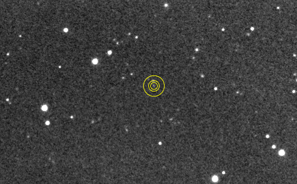
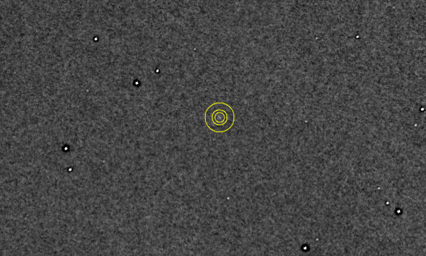
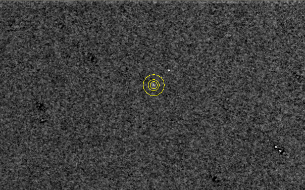
Figure 5. Top Image: Median
combine of three 180-second exposures with standard calibration
(cropped to 9.8 x 6.1 'arc). The brightest star to the left of the asteroid (cicled) has V = 14.3. Middle Image: Result of image
subtraction using the procedure described in an earlier section. Bottom Image:
Obtained by median combining the
previous image with 3 others that were processed the same way.
The "offset alignment dot" can be seen to the upper-right of the
asteroid.
At each
stage of the image subtraction and median combining process the stars
become fainter and the
asteroid stands out more with undiminished flux. The limiting
magnitudes for these clear-filter images are 21.5 for g = 12 minutes,
and 22.5 for g = 48 minutes. FWHM varied from 3.0 to 3.5 "arc for
3-minute exposures (AO-7 tip/tilt image-stabilized). The magnitude
scale is well-established since the uncropped images are of a star
field containing Skiff catalog stars with BVR magnitudes. (According to
MP Checker there is no asteroid at this location.)
Related Links
Minor Planet Bulletin article describing image subtraction
Image stacking w/o image subtraction
A More Detailed Version of image subtraction for asteroids
Another example of an asteroid light curve using image subtraction
Astrophotos web page
__________________________________________________________
First created: 2005.10.07 Last updated: 2006.03.30