Image Subtraction Procedure for Faint Asteroids
Bruce L. Gary
Links Internal to this Web Page:
Introduction
Rotation Light Curve
Images Illustrating Image Subtraction Concepts
Brief Image Subtraction Procedure
Detailed Image Subtraction Procedure
Related Links
Introduction
This image subtraction procedure is a slightly improved version of the one described in the Minor Planet Bulletin article: Gary, Bruce L. and David Healy, "Image Subtraction Procedure for Abserving Faint Asteroids," Minor Planet Bulletin, 33, 1, pg 16-18, 2006 January-March (the issue is available for download at MPB; the article is available as a web page at MPB art web page version).
This web page uses observational data taken 2006.01.28 of the asteroid
86279, which bears the official name "Brucegary." Thanks Dave Healy and
Jeff Medkeff, for discovering this asteroid (in 1999) and for giving it
my name.
Rotation Light Curve Results - to Date
This graph shows results, to date (2006.02.08), of my attempt to create
a rotation light curve based on the image subtraction procedure for
asteroid "86279 Brucegary."
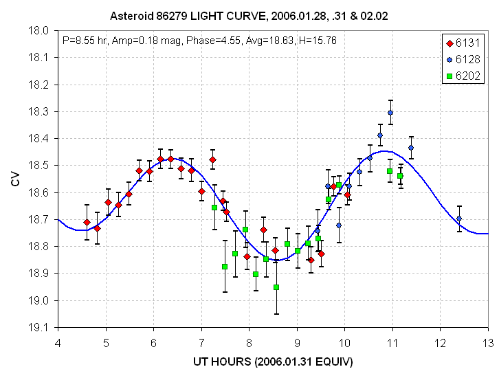
Rotation light curve (preliminary and incomplete) based on 3 observing dates.
Note the difference in briughtness of the two minima (en-on views).
This difference is most likely produced by uneven shapes of the
opposite ends. Backscatter of sunlight varies strongly with slope; so
the end-on view at 8.5 UT must have a more angular shape than the 4.5
UT end view.
Images Illustrating Image Subtraction Concepts
The basic concept is to get a star field image taken when the asteroid
is somewhere else and subtract it from the same star field when the
asteroid is present. This "removes" the stars while leaving the
asteroid at 100% of its actual level. This subtracted image is then
used to measure the asteroid's brightness. Sounds simple, but there are
a few details along the way.
One detail has to do with cosmic ray artifacts in the CCD image. For
example, here's a 4-minute exposure with a couple dozen cosmic ray
defects.
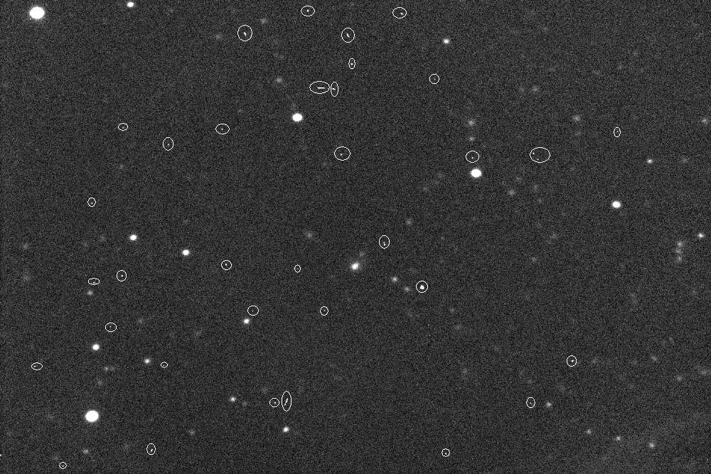
Figure 1. Example of cosmic ray defects (circled) in a 4-minute exposure (image #49).
The best way to eradicate these artifacts is to "median combine" 3 (or
more) images of the same star field. Here's an example of this.
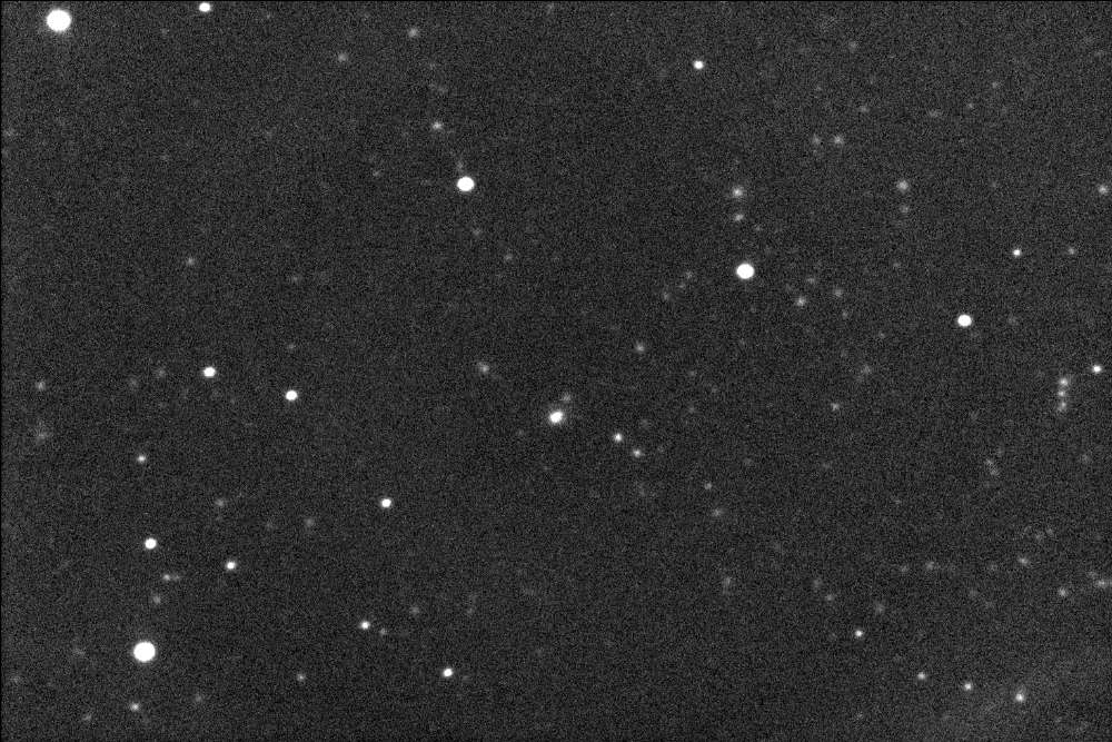
Figure 2. Median combine of previous image with two of its neighbors.
Note that in this median combine of 3 images there are no cosmic ray
defects. Also, the stars appear brighter becasue the background noise
has been avered down.
There's only one problem indoing this. The asteroid moved during the 12
minutes required to take the raw images, so it appears as an oval
whereas the stars are circular. This can be overcome by doing another
median combine of the same 3 images, but with offsets introduced to
compensate for the asteroid's motion.
This last step is easier said than done. You have to pixel edit an
artificial star (just a white dot will do) in each image at a location
that is offset from a reference star by amounts calculated from the
asteroid's rate of motion and time between images.
Provided there are no stars near the asteroid that could interfere with
the photometry measurement of its brightness the rest of the analysis
is straightforward. You just measure the "flux" from the asteroid
(using an aperture size that captures most of the asteroid's image),
and convert flux to magnitude (using equations described elsewhere).
Faint asteroids always have background stars too close to it that they
interfere with the asteroid's flux measurement. That's a problem for
image subtraction.
The first step for image subtraction is to create a master image for
subtracting from the individual asteroid images. One way to do this is
to median combine all images of the star field taken during an
observing session. For the case study used here (2006.01.28 UT), I have
34 images, each a 4-minute exposure of the same star field. A median
combine of these 34 images produces a "deep" image without cosmic ray
artifacts and with almost no trace of the asteroid (since it was
moving).
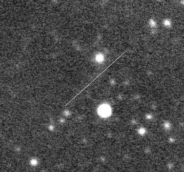
Figure 3. Median combine of 34 images, and cropped to show
only the region surrounging the asteroid's path (line) during the
3-hour observing session. The image scale is different from the
previous images.
This 34-image median combine has much less sky background noise than
the individual images. Therefore, subtracting it from the individual
images will have minimal effect on the noise level of the subtracted
image. However, it has one defect we want to overcome: there's a
slightly brighter band along the asteroid's path in the 34-image median
combine. This was expected since even median combining gives a slight
"bright bias" to locations that are bright in only one image.
Therefore, it is advisable to create about 3 master star field images:
one for use during the first 1/3 of images, another for the middle 1/3
and one for the last 1/3. For example, the one for use with the middle
1/3 of individual images can be a median combine of images from the
first 1/3 and last 1/3. This reduces the "bright bias" considerably,
and assures that the eventual "rotation light curve" will not be
influenced by the image subtraction process.
Once a set of 3 master star fields are prepared they must be subtracted
from all individual images (using the appropriate master image for each
individual image). Here's how the image of Fig. 1 turned out
after image subtraction.
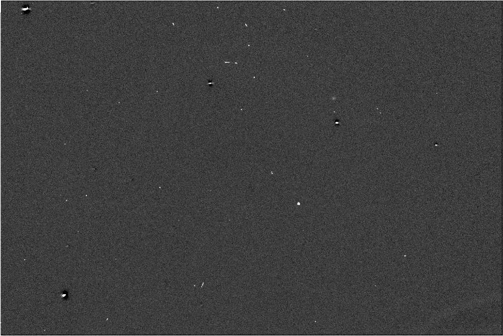
Figure 4. Image #49 (same as in Fig. 1) after subtracting a
master star field image. The cosmic ray artifacts are still present,
and only a ghost image of the 4 brightest stars is present (but at a
much reduced level). The asteroid can be seen in the upper-right
quadrant, north of the brightest ghost star feature.
After this image's two neighbors were "images subtracted" they were median combined to create the following image.
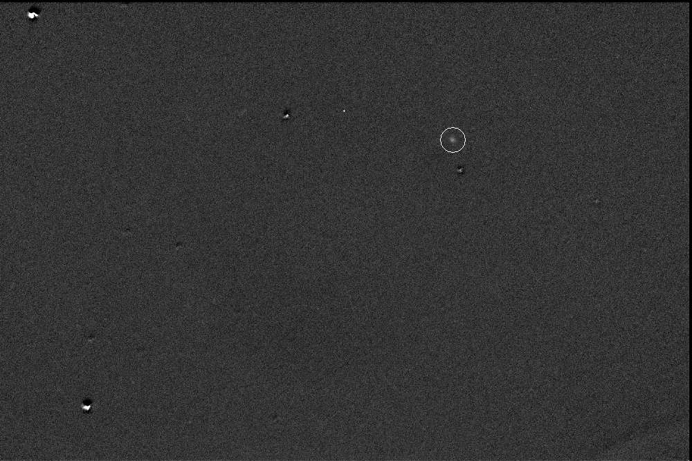
Figure 5. Median combine of the image in Fig. 4 and two
neighbor images, all of which were subjected to the "image subtraction"
process. The asteroid (circled) is present and there are no cosmic ray
artifacts. The small white dot above the image center is an alignment
dot used to correct for asteroid motion.
As the caption suggests the above image was a median combine of 3
subtracted images using an alignment dot to correct for asteroid
motion. The alignment dot was placed in the images before subtracting
the master image. This is necessary because the alignment dot is pixel
edite dinto the image at a location that is carefully offset from the
centroid location of a reference star, and the reference star
essentially disappers after image subtraction (or its ghost artifact is
mis-shapen and can't be used for position offsetting). This is the most
tedious part of the process. To pixel edit an alignment dot you have to
note the time of the exposure in a spreadsheet, then enter a reference
star's x,y location in the individual image (before subtraction), then
calculate the x,y location of the alignment dot using an estimate of
the asteroid's rate of motion in x and y.
There's another subtlety that should be dealt with: when measuring the
flux of the asteroid in an image like that depicted in Fig. 5 it is
important to use a carefully chosen photometry aperture size and a
"recovery factor" that was determined for that aperture. This requires
an extended explanation.
When a photometry aperture size is varied the fraction of counts that
are "recovered" varies; when the aperture size is large nearly 100% of
the counts are recovered. That large a recovery factor would be good if
it didn't come with a signal-to-noise (SNR) penalty. By decreasing the
aperture the SNR improves, reaching a maximum, then decreasing again as
aperture size approaches zero. The reason for this has to do with the
noise in each pixel due to the sky background level and the process of
reading the pixel value after an exposure has been completed. The noise
within the photometry aperture increases as the square-root of the
number of pixels within the aperture area, or noise is proportional to
the aperture radius. The maximum SNR is achieved when the aperture
radius = 75% of the FWHM (assuming the point-spread-function is
Gaussian). For reasons that are not worth going into here it is wise to
choose an aperture radius that is slightly larger than the one that
yields maximum SNR (it has to do with systematic errors). When, for
example, aperture radius = FWHM the measured flux (measured as counts)
is about 93% of the flux that would be measured with a large aperture.
For this situation the "recovery factor" is said to be 0.93. Knowing
this allows the faint object's "full flux" (large aperture flux)
to be calculated using the aperture yielding the (almost) best SNR by
simply dividing the measured flux by the recovery factor. This is like
"having your cake and eating it too."
These concepts may be straight forward but implementing them is not.
For example, how can you determine a recovery factor for a subtracted
image? You can't. So you have to use a median combined image using
images that haven't been image-subtracted. That can be done using the
same 3 images that will make the Fig. 5 image but before they are
image-subtracted they are median combined using stars for alignment.
The FWHM of a point source in the star-aligned image should be the same
as the asteroid's FWHM in the Fig.5 image (that used the alignment dot
for alignment).
Brief Version of Image Subtraction Procedure
This "brief version" of the procedure I use for image subtraction
emphasizes the concepts verbally described in the previous section. A
detailed version is given later.
1) Calibrate all raw images (dark frame and flat frame).
2) Measure the UT start time, reference star x,y location, reference star FWHM and flux.
3) Check image quality (sharpness and flux) for all images; select groups of 3 for later combination.
4) Calculate an x,y location for the alignment dot for all iamges; pixel edit them into all images.
5) Median combine all "groups of 3" using star alignment.
6) For each star-aligned group of 3 image measure a faint star's SNR for various choices of aperure size.
7) Choose an aperture size that is one step larger than the one that gives maximum SNR.
8) Use a bright unsaturated star in an uncrowded field to determine recovery fraction for the chosen aperture size.
9) Create the 3 master star field images by median combining
large numbers of images that don't have the asteroid in specific parts.
10) Subtract the appropriate master star field image from all individual images.
Note: Use a
reference star to align the two images; rescale the intensity of the
master image so that it's reference star has the same flux as in the
individual image.
11) Median combine the "groups of 3" subtracted images using the alignment dot.
12) Measure the asteroid's flux using the aperture size chosen in step 7 (for that "group of 3").
13) Adjust the asteroid's flux by the recovery factor, making it
equivalent to what would have been measured if a large aperture size
had been used.
At this point in the analysis you have to decide whether to convert
asteroid flux to magnitude using an all-sky method or a differential
photometry method. If the sky is judged to be cloudless during the
entire observing session then it is easier to use the all-sky method.
If cirrus came and went, then you'll have to rely on a differential
photometry method.
All-sky analysis path:
14) Determine the air mass for each individual image using its exposure
start time plus half the exposure time and a "planetarium program" -
such as TheSky.
15) Enter the asteroid's flux, recovery factor, exposure time, and air
mass into a spreadsheet, such as Excel. Calculate asteroid magnitude
using "simple magnitude equations."
Note: An
explanation for Simplified Magnitude Equations can be found at SME.
Differential photometry analysis path:
14) Determine a reference star's large aperture flux for each "group of 3" star-aligned (un-subtracted) image.
15) Enter the reference star's flux in the spreadsheet. As an option
you may create an extinction plot to verify that cirrus clouds were a
problem.
16) etc. It's all described at my SME web pages.
If you think this procedure is daunting, wait until you see the detailed version of what I do. Read on.
Detailed Version of Image Subtraction Procedure
The previous section was meant to emphasize the concepts employed by
the "image subtraction" procedure. In this section I present a detailed
list of steps I currently use for implementing image subtraction.
In the following the term "XLS" is used to refer to a spreadsheet. When
I say "note" I mean write down the information in a reduction log and
enter into XLS. It is assumed that there's a master flat and master
dark for the images to be processed. I use the term "triplet" to refer
to 3 images taken close in time that are to be used for median
combining. Before processing the images determine the asteroid's rate
of motion (available from an ephemeris, or use a planetarium program,
or measure images from beginning & end).
1) Start with a the first group of 3 acceptable images;
calibrate them (dark frame, flat frame, flatten, hot pixels 10%). Don't
use bad quality images (tracking trailed, seeing bloom).
2) Select a bright (unsaturated) star for use as a position reference and flux reference.
3) Median combine using star alignment; save as 565758_mcs (where the 3 images are 56, 57 & 58).
4) Set the aperture circle big & measure a reference star's
flux, S*; note the star's FWHM and flux in the reduction log.
5) Choose a small aperture radius (larger than the one yielding
maximum SNR by a couple pixels) and note its radius & flux recovery
fraction (fa = flux using small aperture, radius a, divided by flux
using larger aperture).
6) For each of the 3 images note the UT mid-time; note the reference star's big aperture flux, FWHM and x,y location.
7) Use TheSky to determine air mass values for each image.
8) Enter in XLS each image's UT, FWHM, flux, x/y location and
air mass; note XLS's calculated offset x/y location for the alignment
dot.
9) Pixel edit a white alignment dot at the calculated x/y
location; save the image as 56_dot. Repeat for the other 2 images.
10) Move the image files just created to respective directories.
11) Repeat above for all raw image files.
12) Median combine the last 2/3 of mcs-files for later use as a master
star image for the first 1/3 dot files; save as MSI_A. Median combine
the first and last 1/3 for later use with the middle 1/3 of dot files;
save as MSI_B. Median combine the first 2/3 of mcs files for later use
with the last 1/3 of the dot files; save as MSI_C.
13) Determine extinction by plotting step 3's reference star flux (S*) vs air mass. Manually solve for slope [mag/airmass].
14) If there are observations of standard star fileds, such as Landolt
areas, process them (see SME web page). Note SME constants (zero shift,
extinction & star color sensitivity).
15) Load the 3 image members of the first calibrated image "triplet." Load the appropriate MSI.
16) Consider sharpening or smoothing the MSI image to achieve
similarity of its reference star FWHM and the average FWHM of the 3
triplet images.
17) For each image of the triplet align the MSI image with that
individual triplet member. (With MaxIm's align tool select the triplet
image first, then the MSI image).
18) Subtract the sligned MSI image from the triplet member image. (With
MaxIm's pixel math tool, highlight the triplet member image, invoke the
tool, select the MSI image for subtraction, set the scaling for the
triplet image to 100%, set the scaling for the MSI image to 100% *
Striplet / Smsi).
19) Save the image subtracted triplet member image as 56_dot_is.
20) Undo the sharpening or smoothing performed on MSI in step 16.
21) Repeat steps 16 to 20 for the other two triplet member images.
22) Median combine the 3 "image subtracted" triplet image members using the alignment dot. Save as AST_565758.
23) Measure the asteroid's flux, Sa, using the aperture radius noted in
step 5. Note and enter the flux & SNR in XLS. The recovery factor
associated with the aperture used for emasuring the asteroid's flux was
determined in step 5; enter this in XLS (at the row for the triplet).
24) Repeat steps 12 to 23 for all triplets.
25) In XLS, for each triplet row adjust the asteroid's flux by the
recovery factor, making it equivalent to what would have been measured
if a large aperture size had been used.
26) Use the SME equation and constants (determined for the observing
session) to convert asteroid triplet flux, air mass
& recovery factor to CV magnitude. Use a default
asteroid star color of C = 0.09 (based on V-Rc = 0.40, or B-V = 0.69;
as the SME web page states C = V-Rc - 0.31, which is equivalent to 0.57
* (B-V) - 0.30).
27) Plot asteroid brightness, CV, versus time, etc.to obtain a portion of the asteroid's rotation light curve.
That's all! I'm aware that probably nobody enjoys data analysis as
much as I do and the image subtraction procedure described above will
never be used by anyone else. My purpose in presenting this detailed
procedure on this web page serves as a record for my later reference,
in case I take a break from doing faint asteroid light curves and later
come back to doing it but have forgotten some of the steps.
Related Links
Minor Planet Bulletin article describing image subtraction
Stacking w/o image subtraction
Another image subtraction tutorial
A tutorial for median combining using an asteroid alignment dot but without image subtraction
Asteroid light curve using image subtraction (asteroid 86279)
Another description of image subtraction (asteroid 46053)
Astrophotos web page

__________________________________________________________
First created: 2005.06.29 Last updated: 2006.02.08