Asteroid Hunting
Bruce L. Gary, Hereford Arizona Observatory (G95)
Overview
Asteroid hunting, or trying to discover an asteroid that's not already
cataloged, is a big challenge for anyone using a telescope with an
aperture smaller than 20 inches. This generally acknowledged wisdom,
while true, does not mean that someone with only a 14-inch telescope
can't discover an asteroid. The smaller telescope just means that the
search will be "labor intensive" in both observing and image analysis
compared with using a larger telescope for which observing and image analysis are
relatively stratightforward. This web page explains what must be dealt
with by the small telescope user wishing to try for an asteroid
discovery.
I have two purposes in creating this web page: 1) explaining a thing
helps me understand it better myself, and 2) having spent a lot of
effort to derive an insight into relevant factors that should influence
an observing and data analysis strategy, I want to share these insights
with other amateurs who might be floundering the way I have with the
same problem.
The Goal
The Minor Planet Center, MPC, requires that for two
dates, preferably one or two days apart, positions of a candidate new
asteroid be submitted that can "link" together with ressiduals of no
greater than 1.5 "arc for all positions. Although magnitude estimates
are not required it will be helpful for you as an observer to know how
you're performing (SNR and residuals) for the magnitude range where you
should be searching. As explained in the next section, you need to be
capable of measuring the positions of asteroids fainter than 20th
magnitude since almost all brighter asteroids have been cataloged.
Undiscovered Asteroid Statistics
There are more than a million asteroids already cataloged with known
orbits and approximate brightnesses. A model for asteroid size
distrribution and orbit sizes has been used to create a model for the
total number of asteroids (discovered plus undiscovered) that are
present in the night sky. This is shown in the next figure.
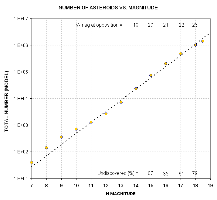
Figure 1. Total number of asteroids versus brightness at the standard distance of 1 a.u. (for opposition illumination and viewing).
Numbers at the top are approximate magnitude at opposition (assuming a typical main belt orbit). Data from Bidstrup et al (2004).
By comparing
statistics for the already discovered asteroids with what would be
expected using the model just referred to it is possible to estimate
how many
asteroids of any given size (brightness) remain undiscovered. This is
shown in the next figure.
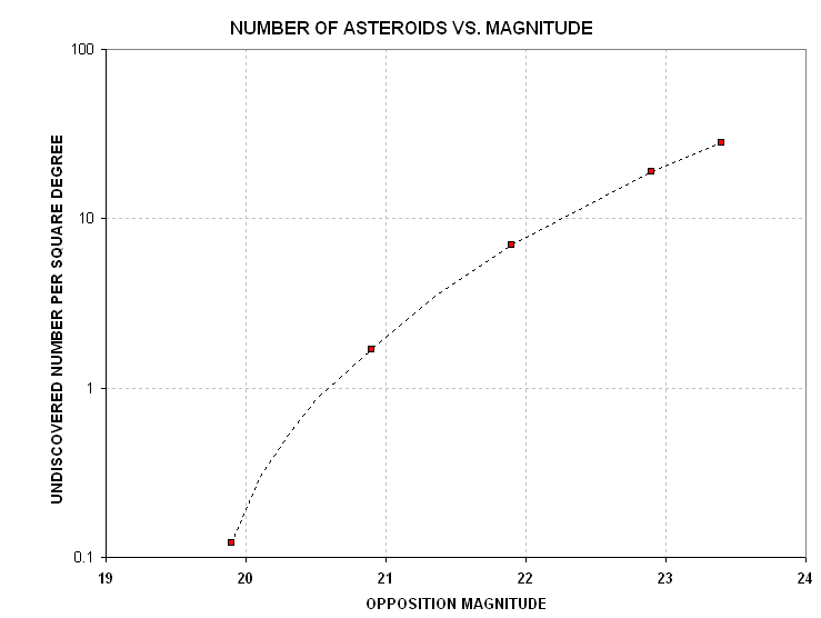
Figure 2. Total number of "undiscovered asteroids" versus brightness at opposition (assuming a typical main belt orbit).
The number of undiscovered asteroids brighter than V-mag = 20 is less
than one per 10 square degrees, and the number becomes vanishingly
small for brighter asteroids. This is why the goal for discovery is to
be able to detect and measure the position of asteroids fainter than
20th magnitude.
Notice that there's an approximate 10-fold increase in the number of
undiscovered asteroids in going from V-mag = 20.0 to 21.0. The rewards
for "going deep" are great. But so are the rewards for having a large field-of-view (FOV). As will be see below, striving for one payoff causes a loss in the other.
Limiting Magnitude
Limiting magnitude is usually defined as the V-magnitude of a
point-source that produces a signal-to-noise ratio (SNR) of 3.0. As a
practical matter when someone is asked to visually inspect an image and
indicate an example of the faintest star in the image it will turn out
toi have SNR of about 6, not 3. The following figure shows
limiting magnitude, ML, for a 14-inch Celestron.
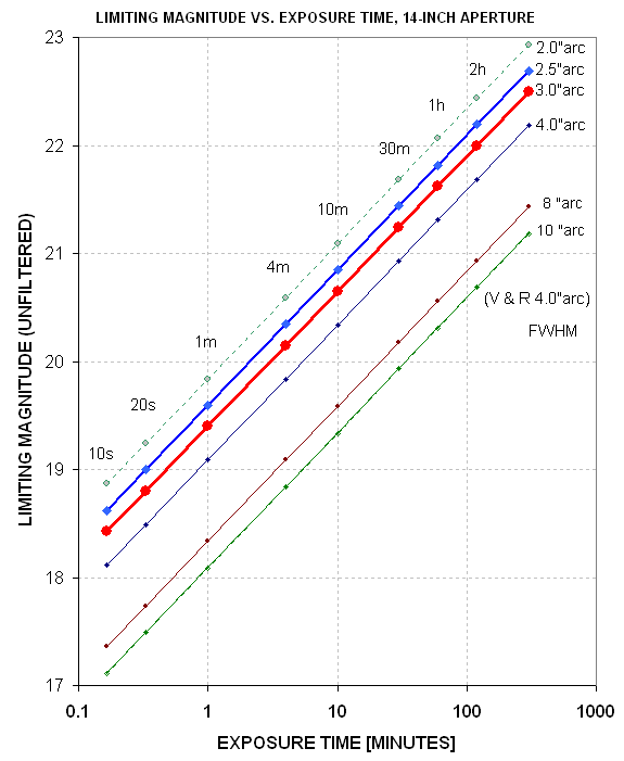
Figure 3. Limiting
magnitude (unfiltered) versus total exposure time and FWHM
("atmospheric seeing"), derived empirically using an SBIG CCD and a
clear filter. It is assumed that moonlight is not present (and there is
minimal light pollution from nearby cities).
Notice that there's strong dependence of ML
upon the half-power diameter of stars in the image (FWHM). Usually,
FWHM is determined by "atmospheric seeing" but for a prime focus
configuration, or a Cassegrain configuration with 2x2 or 3x3 binning,
the value for FWHM may be so large that it is relatively unaffected by
atmospheric seeing. For example, my Celestron at prime focus (using a
Starizona HyperStar field flattening lens) produces star images that
have FWHM ~9 "arc (7.2 "arc for the best seeing and 10 or 11 "arc for
the worst seeing). At prime focus the image scale is 2.8 "arc/pixel, so
even with perfect optics and no atmospheric seeing degradation the best
possible FWHM would be ~5 "arc. Cassegrain configurations can employ a
focal reducer lens for enlarging the FOV. With a 3.3x Celestron focal
reducer attached to the back of the telescope the FWHM is typically ~3
"arc, whereas without the focal reducer it is typically 2.5 "arc. (My
site is at 4650 feet altitude in Southern Arizona.)
In the figure the term "Exposure TIme" refers to the total exposure
time of all images used to produce the image whose ML is being
described. Every time an image is "read out" from a CCD "read noise"
isadded to the noise that existed before read-out. Therefore, a one
hour exposure will have a deeper ML than the combination of 60
one-minute images. Combining images can be done by averaging or median
combining, and this choice will affect the final image's ML. These are
some of the reasons that the slope of the lines in this figure do not
agree with the theoretical slope that would exist for making just one
exposure for the indicated time; instead, the slope is based on
empirical data, using typical observing and image combining procedures.
It is important to understand why FWHM is so important in setting ML. I
am assuming the user employs aperture photometry with the signal circle
diameter equal to ~ 2.0 times FWHM. This is larger than the
theoretically best SNR choice of 1.5 times FWHM, and it is prudent to
not use anything smaller than ~2.0 so that small changes in a star's
point-spread-function (PSF) will have negligible effect on the measured
star flux. Note that PSF shape and size is likely to vary across an
image, especially if the f-ratio is small (for Prime focus my f-ratio
is 1.86). The PSF will also vary from images ot image due to seeing
changes and focus setting errors. When FWHM is small, the number of
pixels containing the star's signal will be small, and this allows the
user to set the photometry signal circle to a smaller number of pixels.
Since each pixel has "noise" (attributable to thermal effects in the
instrument as well as temporal fluctuations of the sky background
level) the smaller the number of pixels within the signal aperture the
greater the ratio of star flux to noise. When FWHM is doubled, the area
of the signal aperture must be quadrupled. This will lead to a doubling
of noise due to stocahstic processes (such as thermal noise and sky
background noise). Therefore, a doubling of FWHM causes SNR to be
reduced by a factor of two. This, in turn, is equivalent to a 0.75
change in magnitude.That's what can be seen in the graph, above.
Asteroid Motion and Exposure Times
At opposition an asteroid is moving westward, or retrograde, due to the
Earth's greater orbital velocity. There are locations along the
ecliptic where the asteroid's motion is small, as it switches from
retrograde to prograde, and this is typically at 70 degrees from the
anti-solar point, as shown by the following figure.
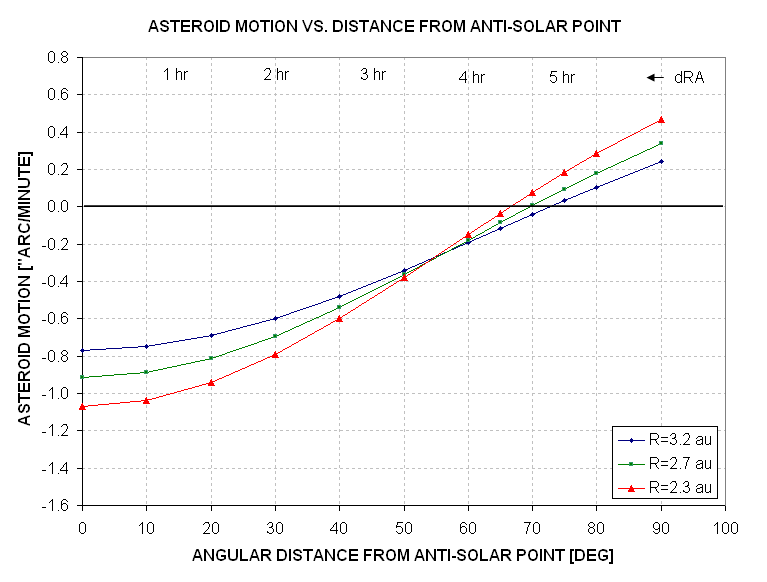
Figure 4. Rate of motion of an asteroid in an uninclined circular orbit versus angular distance from the sun along the ecliptic.
If an asteroid at opposition moves at 1 "arc/minute and if FWHM = 3
"arc, an exposure of 3 minutes would produce an oval shaped asteroid
with dimensions ~4.5 x 3.0 "arc. A longer exposure would yield ever
decreasing improvements in SNR, and ever-increasing problems of
interpretation as well as a greater probability that the asteroid would
be close to a background star that would bias the measurement of its
position and magnitude. My rule-of-thumb is to keep the exposure
shorter than 2/3 FWHM. In this case, the maximum exposure would be 2
minutes.
If the same asteroid were observed when it was ~70 degrees from the
anti-solar point, however, its motion would considerably less. This
would allow longer exposures, but two factors compensate for this gain
of SNR due to a longer exposure: 1) the asteroid is farther from the
Earth, and hence fainter, and 2) it is being viewed at less than full
illumination (i.e., gibbous phase) without the benefit of the
opposition brightening effect, which also makes it fainter. For
example, asteroid 2005 US157 is predicted to be 1.3 magnitudes fainter
when it's at 70 degrees from the anti-solar point than when it's at
opposition. Equivalent exposure times for the two magnitudes (19.8 and
21.2) are 2 and 20 minutes (for SNR = 1 with a 14-inch telescope and
3.0 "arc FWHM). In other words, a 2-minute exposure at opposition,
producing a 2 "arc smearing of the asteroid image in its direction of
motion, will have the same SNR = 1 as a 20-minute exposure when it's at
a location where it's moving much slower. For this specific asteroid
case, chosen at random, it is better to observe it at opposition and
stack 2-minute images in order to produce an image with sufficient SNR
for the accurate measurement of its coordinates. The relationship
between position accuracy and SNR is dealt with in the next section.
Position Accuracy versus SNR
When using PinPoint to plate solve (leading to coefficients that
convert pixel coordinates to RA and Dec coordinates) it is common to
achieve average residuals of 0.1 "arc for a Cassegrain configuration
and 0.2 "arc for a prime focus configuration. These residuals are for
the stars used in the plate solving procedure, which I am assuming are
from the UCAC 2.0 star catalog. When I started observing asteroids I
naievley assumed this average residual would also apply to any asteroid
I had in the image. For bright asteroids this should be correct, but
for faint ones the expected coordiante accuracy must degrade as SNR
decreases. The way to understand this is to imagine the background
level of the image to be a topographic surface with hills and valleys.
The topography bumpiness is caused by sky background noise, CCD readout
noise, thermal noise of the CCD electronics, imperfections of the dark
frame used, and imperfections of the flat field frame used. The fainter
the asteroid the greater these topographic features shift the apparent
centrroid position ffect of the asteroid feature. I have empirically
derived the following equation for for position uncertainty versus SNR:
Position Uncertainty = Star Fit Residuals + 2.2 * FWHM ["arc] / SNR
For example, when SNR is large, Position Uncertainty = Star Fit
Residuals (the thing PinPoint reports as average residual). This makes
sense. But when SNR is small the second term dominates. For example,
when FWHM = 9 "arc (forced high due to the prime focus image scale of
2.8 "arc) and SNR =
15, the average residual is ~1.5 "arc. This "expected average residual"
is the same as the MPC requirement
of 1.5 "arc, and is therefore unacceptable since about half the
position errors will exceed the MPC threshold. A reasonable goal is to
achieve an expected average residual of 1.0 "arc.
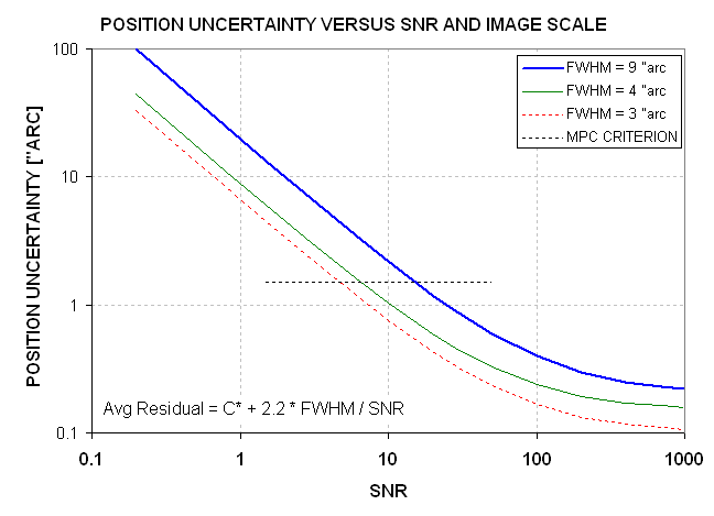
Figure 5. Average residual position uncertainty versus SNR for three image scale values, based on Declination measurements of a faint asteroid on 4 dates.
If small SNR is to be useful it must be accompanied by a small FWHM
and this favors Cassegrain configurations over a prime focus one. For
example, when FWHM = 3 "arc (typical for one of my Cassegrain
configurations) the desired average residual of ~1.0 "arc can be
achieved with SNR = 7.
Image analysis Strategies
I have already described how
each individual image should not be exposed for longer than the time it
takes for the asteroid to move ~2/3
of a FWHM distance against the background stars. Recall that we are
searching for an asteroid that is probably too faint to be seen in any
of the individual images. How, then are we to align the images for
stacking (using either averaging or median combining)? If we use "star
alignment" to register the images the resultant stacked im age will
further smear the asteroid. Although we can't use the asteroid for
alignment we can make use of our knowledge of a typical motion for
asteroids in the part of the sky we're observing. One way to get such a
motion vector is to use the MPC's web page for producing a list of
asteroids in the part of the sky we're observiong. Another way is to
quickly process the bright asteroids in our FOV (in a prime focus FOV I
typically see about a dozen asteroids). The MPC web page
http://scully.harvard.edu/%7Ecgi/CheckMP
allows the user to enterRA/Dec coordinates and retrieve information
about asteroids in that area, including rates of motion in both RA and
Dec.
Once a typical pair of motion rates have been established it is
possible to stack images so that most asteroids in the FOV are
approximately aligned. This can be accomplished by pixel editing an
"offset alignment dot" (OAD) in each image and then combining the
images using a "single star alignment" method where the OAD is the
specified "star." In this way the SNR for most asteroids in the FOV
will increase to the level where they can be "seen." The best way to
"see" the asteroids after this SNR enhancement is to blink two or three
such images (using star alignment, so that the asteroids move). The
procedure for adding OADs is summarized here:
1) Measure the x,y coordinates of a star to be used as an offset reference
2) Note the UT for that image
3) Using a spreadsheet (or calculator) calculate how
much movement a typical asteroid is expected to move in both x and y
4) Add an offset to the above delta-x and delta-y values (so that the OAD will end up in a star free region)
5) Add the results of steps 1 and 4; this is the coordinate for the OAD
6) Pixel edit a "bright" dot at this location in the iamge
7) Repeat the above steps for other images; do this for 8 images, for example
8) Median combine (or average) the first 4 images using the OAD for alignment; repeat for the second 4 images
9) Blink the two new images with enhanced SNR and search for asteroids
Note that if groups of 4 images are combined for the SNR enhancement
the asteroid's SNR will approximately double. This is comparable to
being able to expose 4 times longer without asteroid smear, or observe
for the same time with a telescope having an aperture root-two larger
(i.e, a 14-inch telescope will perform as if it's a 20-inch telescope).
Determining RA and Dec coordinates for an asteroid that's seen only in
a SNR-enhanced image can be difficult. If the stars aren't smeared too
much a PinPoint plate solving should be acceptable. But if the stars
are smeared a lot the asteroid coordinated may be determined by noting
the asteroid's x,y location and then going back to the first image in
the SNR-enhanced set (of 4 images) and reading the RA/Dec coordiantes
for that x,y location. (This works with MaxIm DL; I don't kow about
other programs.)
FOV and Deepness Tradeoffs
In this section I bring
together all the considerations of the previous sections to demonstrate
a trade-off analysis meant to choose the best telescope/CCD
configuration. I'll use my telescope to illustrate specific
configuration options. My hardware consists of a Celestron CGE-1400
(14-inch aperture Schmidt-Cassegrain), a SBIG ST-8XE CCD, a SBIG CFW-8
color filter wheel, a Celestron 3x focal reducer lens, a SBIG AO-7
tip/tilt image stabilizer and a Starizona HyperStar prime focus field
flattening lens. Various combinations are possible, leading to large,
medium and small FOVs, as summarized here (using abbreviations for some
of this hardware):
Config A: Prime focus (HyperStar, CFW, CCD), FOV = 72 x 48 'arc, image scale 2.8 "arc/pixel, FWHM typically 9 "arc
Config B: Cassegrain large FOV (focal reducer,
AO, CFW, CCD), FOV = 24.5 x 16.3 'arc, image scale = 0.96
"arc/pixel, FWHM typically 4 "arc
Config C: Cassegrain small FOV (CFW, CCD), FOV = 12.7 x 8.5 'arc, image scale = 0.50 "arc/pixel, FWHM typically 3 "arc
The longest exposure for individual images (assuming an asteroid motion
of 0.8 "arc/minute, and adopting my 2/3 of FWHM rule) are 7.5 minutes,
3.3 minutes and 2.5 minutes for the three configurations. Note that it
is possible to expose for 1/3 as long and median combine 3 images (to
be rid of cosmic ray defects, or imperfect dark frame subtraction).
Doing this, however, adds "CCD read noise" to each image, and median
combining will add an additional 15% to the background noise level.
Let's now assume that we want to submit 3
positions to MPC, with a UT midpoint spacing of at least one hour.
Let's devote an hour of observation to each position (i.e., calling for
a 3-hour observing session, following set-up time). We shall now pose
the question: What is the probability of discovering an asteroid with
this 3-hour observing session corresponding to each of the three
configurations?
Let's consider Config A. Referring to Fig. 5 we note that for
"Config A" we need SNR >26 to assure position accuracies of <1.0
"arc (for each coordinate). From Fig 3 we learn that a 7.5-minute image
with FWHM = 9 "arc produces SNR = 3 for CV = 19.3. Combining 4 such
images (using the OAD procedure) yields SNR = 6. This set of 4 images
requires 30 minutes of observing, so in one hour we could combine
another set of 4 images to achieve SNR = 8.5. We need SNR = 26 for
position accuracy purposes, but CV = 19.3 produces only SNR = 8.5 in
one hour. To overcome an SNR ratio = 26 / 8.5 = 3.1 we must resort to
asteroids that are 3.1 times brighter (1.2 magnitude). Thus, after one
hour of observing we will have an SNR sufficient to assure 1.0 "arc
positional accuracy for asteroids with CV brighter than 18.1. According
to Fig. 2 there are no undiscovered asteroids this bright. Thus, this
configuration appears to be unuseable for discovering asteroids.
Let's consider Config B.
Referring to Fig. 5 we
note that for "Config B" we need SNR >10 to assure position
accuracies of <1.0 "arc (for each coordinate). From Fig 3 we learn
that a 3.3-minute image with FWHM = 4 "arc produces SNR = 3 for CV =
19.7. Combining 4 such images (using the OAD procedure) yields SNR = 6.
This set of 4 images requires ~14 minutes of observing, so in one hour
we could combine a total of 4 sets of 4 images to achieve SNR = 12. We
need
SNR = 10 for position accuracy purposes, and CV = 19.7 produces SNR =
12 in one hour. We have more SNR than necessary for this magnitude, so
we can convert the extra SNR ratio = 12 / 10 = 1.2 to an asteroids that
is 1.2 times fainter (0.2 magnitude).
Thus, after one hour of observing we will have an SNR sufficient to
assure 1.0 "arc positional accuracy for asteroids with CV brighter than
19.9. According to Fig. 2 there are ~0.13 undiscovered asteroids per
square degree that are brighter than this. Our FOV area is 0.11 square
degree, so for this one observing session we have a probability of
discovering an asteroid of ~0.11 * 0.13 = 1.4%.
Let's consider Config C. Referring to
Fig. 5 we
note that for "Config C" we need SNR >8 to assure position
accuracies of <1.0 "arc (for each coordinate). From Fig 3 we learn
that a 2.5-minute image with FWHM = 3 "arc produces SNR = 3 for CV =
19.7. Combining 4 such images (using the OAD procedure) yields SNR = 6.
This set of 4 images requires ~10 minutes of observing, so in one hour
we could combine a total of 6 sets of 4 images to achieve SNR = 14.7. We
need
SNR = 8 for position accuracy purposes, and CV = 19.7 produces SNR = 14.7
in one hour. We have more SNR than necessary for this magnitude, so we
can convert the extra SNR ratio = 14.7 / 8 = 1.8 to an asteroids that is 1.8 times fainter (0.6 magnitude).
Thus, after one hour of observing we will have an SNR sufficient to
assure 1.0 "arc positional accuracy for asteroids with CV brighter than
20.3. According to Fig. 2 there are ~0.4 undiscovered asteroids per
square degree that are brighter than this. Our FOV area is 0.030 square
degree, so for this one observing session we have a probability of
discovering an asteroid of ~0.030 * 0.4 = 1.2%.
This is discouraging. However, the result is sensitive to the model for
residual uncertainty versus SNR and FWHM, as the next section
demonstrates.
Sensitivty of Result on Position Uncertainty versus SNR Model
Notice that Fig. 5 is based on Declination
measurements of a faint asteroid on 4 dates. The following figure shows
observed residuals for both declination and right ascension.
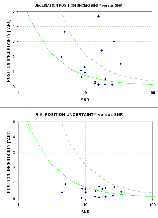
Figure 6. Observed residuals for declination (top pasnel) and
right ascension (bottom panel) for a faint asteroid (CV = 20.3) using a
14-inch telescope in a prime focus configuration (FWHM = 9 "arc). The
grey dashed trace is for Residual = 0.2 + 2.2 * FWHM / SNR, whereas the
green trace is for Residual = 0.1 + 0.7 * FWHM / SNR.
Notice that the top panel has 4 "outliers" (above the grey dashed
trace) out of a total 16 data points. These may have been produced by
faint stars too close to the
asteroid when the image was made that the declination position was
"pulled" away from the asteroid's declination. If this set of data
suffered from "bad luck" then the lower traces should be adopted. If
the four outliers can be identified as outliers by the observer before
they're submitted for MPC to evaluate, such as by their unusual
brightness compared to other readings, then they can be rejected by the
observer before submission. Since I do not yet know if these are
outliers that can be identified by the observer before submission to
MPC it is prudent to consider the more optimistic green trace for
evaluating the feasiblity of discovering asteroids with a small
telescope. It may be worth the effort of employing a technique of
"image subtraction" to remove interfering stars (Gary and Healy, 2005).
On the assumption that the outliers can eventually be dealt with I will
repeat the analysis of the
previous section using the green trace model, as shown for 3 different
FWHM values in the next figure.
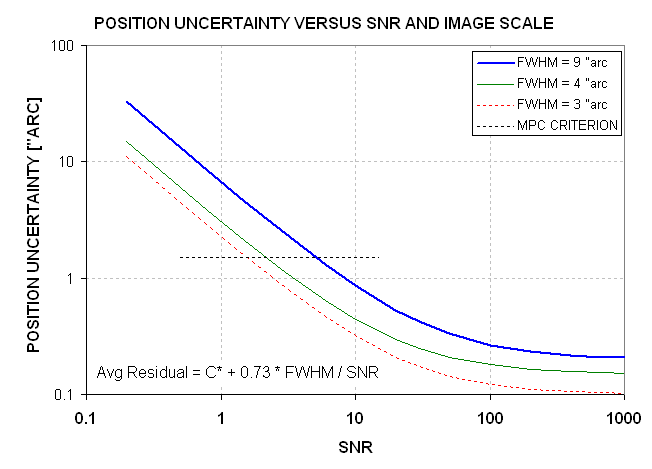
Figure 7. Revised (optimistic) relationship between average residual position uncertainty and SNR for FWHM values 9, 4 and 3 "arc.
These traces can be described by the following equation:
Average Residual Position Uncertainty = Star Fit Residuals + 0.73 * FWHM ["arc] / SNR
Config A: Referring to
Fig. 7 we note that for "Config A" (FWHM = 9 "arc) we need SNR >9 to assure
position accuracies of <1.0 "arc (for each coordinate). From Fig 3
we learn that a 7.5-minute image with FWHM = 9 "arc produces SNR = 3
for CV = 19.3. Combining 4 such images (using the OAD procedure) yields
SNR = 6. This set of 4 images requires 30 minutes of observing, so in
one hour we could combine another set of 4 images to achieve SNR = 8.5.
We need SNR = 9 for position accuracy purposes, but CV = 19.3 produces
only SNR = 8.5 in one hour. To overcome an SNR ratio = 9 / 8.5 = 1.1
we must resort to asteroids that are 1.1 times brighter (0.1
magnitude). Thus, after one hour of observing we will have an SNR
sufficient to assure 1.0 "arc positional accuracy for asteroids with CV
brighter than 19.6. According to Fig. 2 there are might be 0.02 undiscovered
asteroids per square degree that are brighter than this. Our
FOV area is 0.96 square
degree, so for this one observing session we have a probability of
discovering an asteroid of ~0.96 * 0.02 = 2%. After observing 50 such
sky areas there will be an approximate 50% probability of discovering
an asteroid.
Config B:
Referring to Fig. 7 we
note that for "Config B" (FWHM = 4 "arc) we need SNR >3.3 to assure
position
accuracies of <1.0 "arc (for each coordinate). From Fig 3 we learn
that a 3.3-minute image with FWHM = 4 "arc produces SNR = 3 for CV =
19.7. Combining 4 such images (using the OAD procedure) yields SNR = 6.
This set of 4 images requires ~14 minutes of observing, so in one hour
we could combine a total of 4 sets of 4 images to achieve SNR = 12. We
need
SNR = 3.3 for position accuracy purposes, and CV = 19.7 produces SNR =
12 in one hour. We have more SNR than necessary for this magnitude, so
we can convert the extra SNR ratio = 12 / 3.3 = 3.6 to an asteroids
that
is 3.6 times fainter (1.4 magnitude).
Thus, after one hour of observing we will have an SNR sufficient to
assure 1.0 "arc positional accuracy for asteroids with CV brighter than
21.1. According to Fig. 2 there are ~2.5 undiscovered asteroids per
square degree that are brighter than this. Our FOV area is 0.11 square
degree, so for this one observing session we have a probability of
discovering an asteroid of ~0.11 * 2.5 = 27%. Two observing sessions
should produce an approximate 50% probability for success in
discovering an asteroid.
Config C:
Referring to
Fig. 7 we
note that for "Config C" we need SNR >2.4 to assure position
accuracies of <1.0 "arc (for each coordinate). From Fig 3 we learn
that a 2.5-minute image with FWHM = 3 "arc produces SNR = 3 for CV =
19.7. Combining 4 such images (using the OAD procedure) yields SNR = 6.
This set of 4 images requires ~10 minutes of observing, so in one hour
we could combine a total of 6 sets of 4 images to achieve SNR = 14.7.
We
need
SNR = 2.4 for position accuracy purposes, and CV = 19.7 produces SNR =
14.7
in one hour. We have more SNR than necessary for this magnitude, so we
can convert the extra SNR ratio = 14.7 / 2.4 = 6.1 to an asteroids that
is 6.1 times fainter (2.0 magnitude).
Thus, after one hour of observing we will have an SNR sufficient to
assure 1.0 "arc positional accuracy for asteroids with CV brighter than
21.7. According to Fig. 2 there are about 5 undiscovered asteroids per
square degree that are brighter than this. Our FOV area is 0.030 square
degree, so for this one observing session we have a probability of
discovering an asteroid of ~0.030 * 5 = 15%. After 4 observing sessions
of different star fields near the ecliptic there should be an
approximate 50% probability of discovering an asteroid.
The "winner configuration" is "B": Cassegrain
large FOV (focal reducer, AO, CFW,
CCD), FOV = 24.5 x 16.3 'arc, image scale = 0.96 "arc/pixel, FWHM
typically 4 "arc. This was also the winning configuration under the
more pessimistic residual uncertainty model. But there's a large
difference in feasibility between the two models.
Tips for Going Deep
Moon: Moonlight can reduce limiting magnitude by 1 or 2
magnitudes, so serious asteroid hunting should be restricted to times
when the moon is below the horizon. If you really want to try to
observe in the presence of moonlight then use an R-band filter, since
the degradation is significantly reduced. There's a SNR penalty for
using an R-band filter instead of a clear filter, and for my system it
varies from 0.36 at low air mass (m=1.2) to 0.39 at high air mass
(m=3). I-band is not worth it although it's relatively unaffected by
moonlight; the SNR penalties are ~0.24 for all air masses.
Darks: Calibrating with a dark frame (or master dark frame) adds
noise to the light frame image. Therefore, lots of darks are a must
when trying to "go deep." One or two dozen should be enough for the
master dark frame to not add significantly to the background noise
level during the calibration process. I prefer to devote at least a
half-hour to dark frames on every night that I'm doing serious
observing, and I make sure the darks are all at the same CCD
temperature as the asteroid "light" frames. It is well known by
observationalists that for the case of no change in star field pixel
location you should spend as much time taking dark frames as light
frames; the only reason to take fewer darks than lights is that the
star field moves with respect to the field of pixels between exposures.
Flats: Flat frame calibration adds noise, so there are only two
reasons for doing it: 1) when there are dust donuts that could
interfere with the measurement of an asteroid's position or flux, and
2) when you want to achieve an accurate brightness measurement, or
variation of brightness with time during an observing session (as in
"rotation light curve"). For asteroid work, where brightness accuracy
is not important (i.e., when it's OK for accuracy to be no better than
5%, or 0.05 magnitude), it is not important to have an accurate flat
frame but it is important to have a precise one. OK, that needs
explanation. Making a flat frame that is precise is easy: you just set
the focus to what it should be and average, or median combine, lots of
images of a uniformly illuminated white screen (or the zenith sky at
sunset with a couple T-shirts over the aperture). A master flat made
from averaging 16 flats has 4 times less noise than an individual flat
frame. The goal is to minimize additional background noise during the
flat frame calibration process.
CCD Temperature: Cooling the CCD reduces thermal noise. For
every 6 degrees C of additional cooling the CCD thermal noise ("dark
current") can be reduced by a factor of two. For example, going from an
uncooled +10 C to a cooled -20 C leads to a 30-fold reduction in the
CCD's thermal noise level. However, the sky background contribution of
noise will be present so there will be diminishing returns by cooling
below a temperature where the two noise levels are comparable. Hence,
when moonlight is present there is less to be gained by cooling than
when the sky is dark. Also, cooling the CCD will have greater payoffs
near zenith than close to the horizon. Professional observatories are
located at dark sky locations, and they can benefit by additional
cooling. That's why they use liquid nitrogen (at -173 C) to cool their
CCD to a constant value near -100 C.
Seeing and Focus: The better the seeing, the deeper you
can go! This point is abundantly clear from Fig. 3. Of course, to take
advantage of good seeing you need to stay well focused. The two factors
work together; for example, good seeing with poor focus is equivalent
to poor seeing with good focus. I use a graph with lines showing how
focus setting changes with temperature. I have different colored lines
for each filter (note: filter parfocality is worse for "fast"
f-ratios). My focus setting can be read as a number (between 0 and
9999) using a wireless focuser (Starizona's MicroTouch). After the
telescope has equilibrated to the ambient air temperature (an hour or
two after sunset) this graph can be a useful guide in maintaining an
approximately correct focus. Every couple hours I interrupt observing
to perform a manual focus check (plotting FWHM versus focus setting,
and plotting by hand). A too-casual attitude about maintaining the best
focus is equivalent to not caring about the cost of buying whatever
aperture telescope and support equipment you have.
Photometry Aperture Size: The best SNR is achieved when the
diameter of the photometry aperture is 1.5 x FWHM. Smaller apertures
not only suffer from a larger SNR, they introduce systematic errors
when attempting to measure brightness (doing "photometry"). To avoid
the introduction of systematic errors in any photometry that might be
attempted it is prudent to use an aperture diameter of about 2 x FWHM.
For faint objects there's another reason for using a larger aperture
than for bright objects, and that has to do with the influence of noise
in the background on the measured flux and location of the faint
object. Using a larger signal aperture reduces this noise biasing. The
lower the SNR the more influence background noise will have on the
pixel placement corresponding to a maximum flux reading. When SNR
<~10 I choose a pixel location corresponding to the "centroid" shown
in MaxIm DL's real-time display; the aperture's pixel location is
always close to the one giving a maximum flux reading (called
"intensity" by MaxIm DL), but it is sometimes not the same and it is my
impression that the centroid location agrees with my visual impression
of the asteroid's location. I can't give quantitative descriptions of
this because I haven't studied it yet and I haven't read about it.
Aperture Recovery Fraction: If astrometry is the only goal then
this paragraph can be ignored. This tip is meant for those who will
want to do photometry of the faint object. Since the object is faint,
you will be using a small signal aperture diameter, ~3 x FWHM. If the
PSF is a perfect Gaussian use of this aperture size will lead to a
reading of ~99% of the flux that's registered in the image. I'll refer
to this fraction as "F" and express it as a %. The PSF is never a
perfect Gaussian, and this means that the aperture circle will recover
an even smaller percentage of what's in the image (the central
obstruction produces a non-Gaussian PSF; image movement during the
exposure adds to this). When diameter ~3 x FWHM it is common for F ~95
to 98%; using 2 x FWHM can prodcue F = 90%. This last F value would
lead to a magnitude error of 0.1 if it is not dealt with properly. I
evaluate fr using a bright star with no others nearby (in the region of
the image close to the asteroid). The asteroid's measured flux can then
be converted to a magnitude using the F value, as illustrated by the
following equation:
CV = 21.35 - 2.5 * LOG ( S / (g * F) ) - 0.15 * m + 0.67 * C
where CV is a clear-filter V-magnitude equivalent, S is measured star
flux ("or Intensity"), g is exposure time, F =s recovery fraction, m is
air mass and C is star color (defined as V-R-0.31, or 0.57 *(B-V)-0.30,
whichever is more convenient). The constants 21.35 and +0.67 have been
determined empirically for my telescope and CCD system (using Landolt
standard stars). The coefficient 0.15 is a zenith extinction
[magnitudes per air mass] for my site, which varies a small amount with
season and has been determined using many flux versus air mass plots.
This "Simplified Magnitude Equation" (SME)is for converting clear
filter observations to a V-magnitude equivalent, and it assumes that
the star's "color" is known. The color parameter C has been defined so
that when the star's color is unknown a good first assumption is that C
= 0 (since a typical star has C = 0). For asteroids the most likely
value for C = +0.19. More information on this method for converting
measured flux to magnitude can be found at http://brucegary.net/photometry/x.htm
Averaging versus Median Combining: Median combining (MC) is
meant to reduce the influence of cosmic ray artifacts and imperfect
dark subtraction defects (caused by using a dark frame with a different
CCD temperature or exposure time). MC does a good job of this, but you
pay a SNR price of about 15% to 20%. Because of this SNR penalty it is
not advisable to MC images that have already been produced by an
earlier stage of MC. You need a minimum of 3 images for the MC to work
(I prefer to use 4 when they're available and when asteroid motion
smearing allows it). If SNR is not a concern, and when asteroid motion
smearing is not an issue, then it's OK to MC a large number of images.
But for maximum SNR it is better to average images. When averaging
instead of MC'g it is prudent to visually inspect each image and reject
those with artifacts near the asteroid. When you want to determine the
asteroid's brightness it is much safer to use averaging instead of MC'g
(and never use the hot pixel removal tool).
Progress Report
So far I've only observed one star field in search of an uncataloged
asteroid (using "Config A"). I "detected" an uncataloged asteroid but
my residuals exceeded MPC's acceptance threshold of 1.5 "arc on the
first 3 dates of observation. The 4th date was excellent, having
residuals of ~0.4 "arc in both coordinates, but by then another
observatory (Catalina Sky Survey) had observed the same asteroid with
acceptably small residuals (using my good observing date and their good
observations to establish an orbit). Technically, the discovery of
"2005 US157" goes to the Catalina Sky Survey, and that's what happened.
But this was a close call, and my luck was probably affected by the
asteroid being too close to interfereing stars on the first three dates
(producing the outliers discussed in the previous section).
Based on this analysis I'm going to try "Cofig B" a couple times and
try to verify the residuals model. Future results will be added to this
web page.
References
Bidstrup, Philip R., Rene Michelsen, Anja Andersen and Henning Haack, Astron. and Astrophys., August 10, 2004.
Gary, Bruce L. and David Healy, The Minor Planet Bulletin, now published. (An extended treatment of the same matter can be found at http://brucegary.net/Ast46053/x.htm
----------------------- SOME OF MY OTHER ASTRONOMY WEB SITES ----------------------
Tutorials
Photometry for Dummies
For several quick/sloppy procedures
Photometry for Smarties
Novel new method (intuitive) for high accuracy
CCD
Transformation Equations Explained And derived (link used
by AAAVSO)
Atmospheric Seeing Degradation
Atmospheric theory & movie demo
Exoplanet Observing
Strategies "How to" suggestions (link used by AAVSO)
CCD
Imaging Tips "How to" suggestions
Photometry
Error Estimation Stochastic, systematic and total SE
(link used by AAVSO)
Miscellaneous
Hardware
"Hereford Arizona Observatory" (G95)
Amateur Counterpart of
HST 3.5-day exposure (mag 22.8 vs 30.7)
The Big Picture
Overview of immense scale of time and space of the universe
AstroPhotos
Pretty pictures
(plus links to many other pages)
Professional and
Personal (everything branches off from this page)
__________________________________________________________
First created: 2005.11.08 Last updated: 2006.03.30