Focal Reducers Degrade Atmospheric Seeing

Focal reducing lenses are used to increase the field-of-viewww (FOV) by increasing the apparent f-ratio of the optical light paths in front of the CCD. Any time you add another optical component into the total light path you should be prepared for performance degradations. Not only does a lens absorb light (decreasing SNR), but a focal reducer will degrade the sharpness of the resulting image. It is generally understood that you should place the focal reducer lens (FR) at a distance from the CCD chip that is close to the distance used in its design. When this is done the sharpness degradation will be minimal. There's a temptation to palce the FR farther from the CCD in order to further increase the FOV. I will present atmospheric seeing versus elevation angle for threeCassegrain configurations types.

The telscope is a Celestron CGE-1400, a 14-inch with Schmidt-Cassegrain optics. The CCD was a SBIG ST-8XE (1530x1020 pixels, 9 micron spacing). One of the configurations employs a SBIG AO-7 tip.tilt image stabilizer. It adds 4.1 inches to the optical path. For all configurations an SBIG CFW-8 color filter wheel was used. The four FR configurations, image scales and FOVs are:

    1) FR 4 inches farther from CCD than designed value         Image Scale = 0.97 "arc/px    FOV = 24.5 x 16.5 'arc
    2) FR at designed distance to CCD                                    Image Scale = 0.59 "arc/px    FOV = 15.0 x 10.0 'arc
    3) No FR, just the CFW & STE-8XE CCD                      Image Scale = 0.46 "arc/px    FOV =  11.7 x 7.8 'arc
    4) No FR, but inclusion of AO-7                                       Image Scale = 0.47 "arc/px     FOV = 12.0 x 8.0 'arc

Atmospheric seeing is usually described using the full-width at half-maximum (FWHM) of the observed point-spread-function (i.e., the width at half max of a stars brightness distribution). The measurements I report are from 4-second exposures used to establish focus. Configureations 3 & 4 appear to be similar so their FWHM measurements are combined.

My observatory, the Hereford Arizona Observatory (G95), hereafter referred to as HAO, is located south of Sierra Vista, AZ at an altitude of 4660 feet ASL. Figure 1 shows my FWHM measurements.

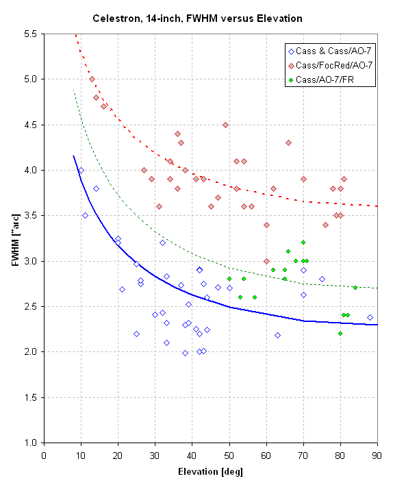
Figure 1. FWHM versus elevation angle for 3 Cassegrain configurations for the HAO site.

The pattern with elevation angle is fitted well by the equation W = C * m ^_a , where W is the fitted FWHM, C is a constant and "m" is air mass (= 1/sin(EL), and "a" is an exponent for air mass. Values for "a" vary slightly with configuration; for the lower two model fits a = 0.30, and for the upper fit a = 0.22.

There's a dramatic FWHM degradation for configuration 1, labelled "Cass/FocRed/AO-7" in the figure legend. Compared to configurations 3 and 4 (No FR) the ratio of FWHM at 50 degrees elevation is 1.52. Considering that limiting magnitude varies in accordance with -2.5 * LOG ( FWHM) this 1.52 FWHM ratio corresponds to a difference in ML = 0.45. That's equivalent to an aperture ratio of 1.23 (i.e., 17.1 vs. 14 inch aperture). It's also equivalent to an observing time ratio of 2.3 (i.e., observing for 23 minutes with FWHM = 3.8 "arc is equivalent to 10 minutes with FWHM = 2.5 "arc). The observing penalties for having the larger FOV are important for some projects.

Notice that placing the FR close to the CFW/CCD, where it should be, incurs a smaller FWHM penalty. The FWHM ratio of 1.16 leads to a limiting magnitude penalty of only 0.16 magnitude (or observing time ratio of 1.34.

While we're looking at this figure notice the big effect that of elevation has on FWHM. The diffference between 20 degrees and zenith corresponds to a limiting magnitude difference of 0.36 magnitude. This is equivalent to an observing ratio of 1.94; it's also equivalent to an aperture ratio of 1.18, or a 16.5-inch at 20 degrees eleavation is equivalent to a 14-inch at zenith).

FWHM versus Time After Sunset

By comparing the measured FWHM with its respective model fit it is possible to search for a dependence of FWHM on "time after sunset." This is shown in the next figure.

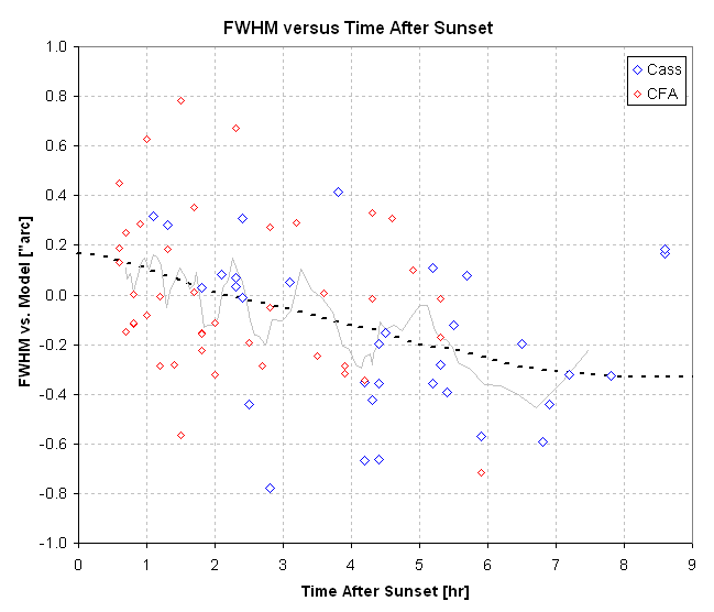
Figure 2. Difference between measured FWHM and the elevation angle model for the appropriate configuration.

This figure suggests a way to model an additional component of FWHM variations, FWHM versus time after sunset. When this model is used for the best configuration (No FR and No AO-7), it is possible to caclulate FWHM at 50 degrees elevation versus time after sunset, as shown in the next figure.

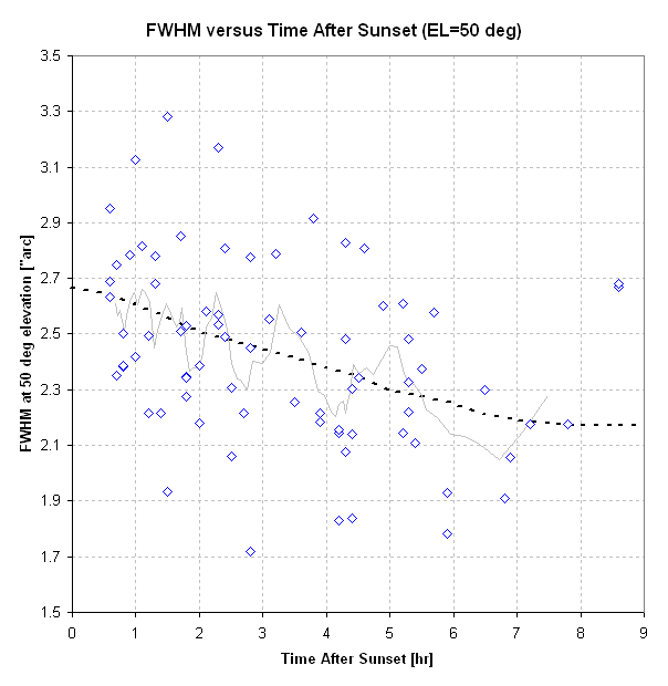
Figure 3. Predicted FWHM corrections for the best configuration and an elevation model, showing the atmosphere's component of FWHM at 50 degrees elevation versus time after sunset. 

There appear to be FWHM payoffs for waiting until midnight to observe. The FWHM ratio of 0.865 corresponds to an improved limiting magnitude of 0.16 magnitude and observing time ratio of 1.34.

Note that for $10,000 you can buy a CCD with 4-times the area of the one I use, and this "solution" affords the same FOV increase as that of the FR in the 4-inch too far ahead configuration. (That's my plan.)

Atmospheric Seeing Demonstration

The following movie demonstrates "atmospheric seeing" using images taken 1/2-second apart with a 10-inch aperture telescope and a Nikon Coolpix 990 digital camera.  There are 11 images, that repeat in a loop at twice the rate at which they were taken.

Figure 4. Animation showing seeing variations on a time scale of 1/2 second.

The large crater on the middle left is Hipparchus, which is about 73 seconds of arc in diameter.  Mars is about 1/4th the diameter of Hipparchus at a typical "opposition" (similar in angular size to the crater at the top of this image that is slightly "cut off" at its top). This quality of "seeing" is typical for an elevation angle of 30 degrees at a sea level site.

If you look carefully you can see that parts of the image move in directions that are uncorrelated with motions at another region. Sometimes a place will appear to magnify, then shrink. Clarity variations (resolution) are the most critical for optical viewing, whereas for astrophotography all the types of distortion produced by atmospheric seeing are important (since image processing normally involves adding several images together).

"Atmospheric seeing" is typically not a problem for "dark sky" objects. It mostly affects planetary and lunar work, since for these objects achieving resolution is far more important than achieving high brightness levels.

"Atmospheric seeing" is caused by non-uniformities of the atmosphere's temperature field. If all atmospheric layers were of uniform temperature, there'd be no "seeing" problems. (Humidity variations are a secondary cause for seeing degradation.)

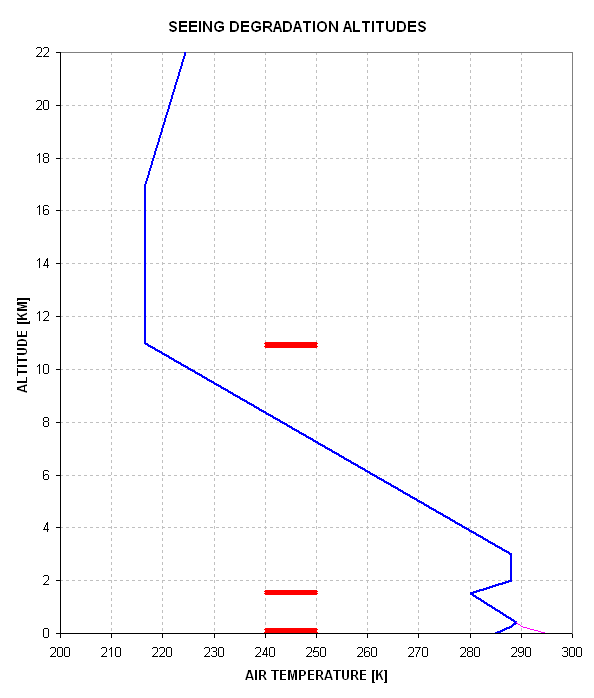
Seeing is usually degraded at three altitude regimes: 1) the surface-based wind shear region (surface to ~40 feet), 2) top of the "planetary boundary layer" (PBL) which can be at 2000 feet, 4000 feet, etc, and 3) near the tropopause, which is at about 36,000 feet (at mid-latitudes) or 52,000 feet in the sub-tropics and tropics (latitudes less than 25 degrees, usually). The first two components of seeing degradation can be greatly reduced by mounting your telescope atop a structure that is at least 15 feet above ground level, or by relocating your telescope to a high altitude site (where something vaguely resembling a PBL is much shallower). The tropopause component of seeing can only be reduced by flying in an airplane at altitudes above the tropopause (i.e., as was done by the Kuiper Airborne Observatory, when it flew out of NASA's Ames Research Center prior to about 1997).

The surface-based component is the most important one, and is described below. The top of the PBL component is second in importance. It should exhibit a small diurnal effect and is probably difficult to predict. A later section is devoted ot it. The tropopause component of seeing does not have a time of day dependence, that I'm aware of, but it does change on timescales of approximately minutes, hours and days.  If the jet stream (located just below the tropopause) is near your observing site, count on bad seeing.  The best seeing is when a high pressure system is centered over the site.  Winds at all altitudes are light at the center of a "high."  If the "high" is off to one side, and the observing site is located where there's a strong pressure gradient, then winds are likely to be strong, producing bad seeing. Winds are never good for seeing, as layers with different wind speeds do not always maintain their laminar flow, and vertical oscillating waves (KH waves) can amplify (and may eventually lead to "clear air turbulence" - which creates disastrous "seeing").

Physical Picture

Turbulence that is not associated with clouds is called Clear Air Turbulence, or CAT.  The parameter crucially related to the generation of CAT is Richardson Number, Ri, which the ratio of stabilizing forces to overturning forces for an atmospheric layer.  The stabilizing "force" is related to buoyancy.  The overturning "force" is vertical wind shear.

When Ri for a layer has a low value, and is sustained at this low value for a long time (approximately minutes), the overturning forces associated with vertical wind shear exceed the restoring buoyancy force and CAT is the end result.  The unstable layer first produces rolling tubes of air.  These rolling tubes eventually breakdown to smaller whirls with random orientations, eventually filling the spatial frequency regime down to centimeter scales.  It's the centimeter scale whirls that can cause atmospheric degradation, ASD; the larger scales just produce image wander (provided another condition, index of refraction vertical gradients, is met, described below).  Before I describe how to calculate Ri, let me give an overview of my understanding of where ASD originates.

Three Layers that Cause Seeing Degradation

There are 3 main layers in the atmosphere that cause most ASD: 1) surface based layer with a scale height of 7 meters, 2) boundary between "planetary boundary layer," PBL, and the free troposphere (the altitude where surface-based convection stops, revealed by cumulus cloud tops), and 3) the tropopause (~11 km).  The first layer is the most important, and the tropopause is the least important.  (Twinkling is produced at the tropopause, but is poorly correlated with ASD.)  Occasionally ASD is produced within layers in the free troposphere, probably where temperature inversion layers exist (marking the boundary between air masses moving in different directions and having different potential temperature, defined below).

Now, since the greatest component of ASD occurs at ground level the challenge for predicting seeing is to predict vertical wind shear, VWS, at ground level.  Topography is all important in determining ground level VWS at a specific site.  Where I live, near mountains, there often are down slope winds after sunset which spread out over my valley in a way that could not be determined from radiosondes, RAOBs, regardless of how close the RAOB site is.  However, ignoring nearby mountain down slope winds for now, PBL winds are moderately well correlated over large regions.  Thus, if you have any measure of PBL wind speed, either from a RAOB not too far away or from an anemometer at your site, you've won half the battle.  This is because the wind profile always goes to essentially zero at the surface (like 1 mm off the ground).  The scale height for this profile is approximately 30 meters, but it depends on topography roughness.  Anyway, the stronger the PBL winds the greater the VWS near ground level, and the greater VWS, the greater is the term in Ri that causes Ri to decrease and approach instability, producing turbulence and ASD.  Therefore, I expect PBL wind speed to be the most correlated parameter with ASD.

Ground Level Vertical Temperature Gradient

The second most important parameter leading to Ri going toward the instability threshold is the vertical gradient of temperature.  After a clear night the ground temperature can be much colder than the air 100 above you.  This will produce a positive temperature gradient, which inhibits turbulence (since an air parcel that rises expands by too small an amount to retain buoyancy).  On a warm, sunny afternoon the surface can be much warmer than the air 100 meters above you.  This is a negative temperature gradient, and invites convection cells to form and produce convection turbulence.  (I forgot to say that there are two kinds of turbulence: 1) VWS-driven, and 2) convection created.)  We can ignore convection turbulence, since it happens in the middle of the day, not at night.  Still, when there's a negative vertical gradient of temperature it's easy for even a small VWS to produce a low Ri and hence turbulence.  So there's an incentive to estimate vertical temperature gradient.  A nearby RAOB would be one solution, though it would have to be in the same topography regime as your site to be valid for you.  Another scheme is to work with surface temperature history.  For example, if tonight is much warmer than last night (and if no fronts have moved through) it's likely that since the air 100 meters overhead changes temperature much slower than the air at the surface you can count on the vertical temperature gradient being more negative than if the surface temperature tonight were not warmer.  On the other hand, if tonight's surface temperature is colder than last night's, and no fronts have moved through (and this could happen when the day was clear and dry, allowing IR photons to radiate to cold space and cool the ground, and nearby air, but not the air 100 meters above), you can count on a more positive temperature gradient than otherwise.

Richardson Number

Now it's time to introduce the formula for Ri.  Ri = dW/dz / dTH/dz, where W is the horizontal wind vector, dz is an increment of altitude and TH is potential temperature, theta, defined theta = T [K] (1000/P[mb])^0.286, where T[K] is the Kelvin temperature of the air and P[mb] is barometric pressure in millibars.  Ri can be simplified in the following way:

     Ri = 9793 [+9.75+(dT/dz[K/km] * (Tstd[K] / T[K])] / T[K] * (dW/dz [m/s per km] )^2

where Tstd [K] is the temperature of the standard atmosphere (288.1 K at sea level) for the altitude in question, z is geometric altitude.  The constants are for a latitude of 30 degrees and an altitude of 0 km.

When Ri , 0.25, and stays at this low value for minutes (?) it is almost inevitable that Kelvin-Helmholtz waves will form and amplify until there is a breakdown of the previously laminar flow and production of turbulence.

Refractive Index Considerations

One more factor should be considered.  It has to do with the refractive index of air.  Light rays bend (refract) when the speed of light is different along one path than a nearby one.  The principal determinants of refractive index are air temperature and water vapor density.  If either is different at two nearby locations (orthogonal to the light path), the light ray path will be bent (refracted). ASD is caused when the refractive index of the air has gradients that are large enough to refract light and when these gradients have different values across the tubular air path from your telescope's aperture through the air to the star.  If turbulence occurs within a layer that has the same air temperature and absolute humidity throughout, it will not cause ASD.  However, it is rare for turbulence to be generated at a layer where there are no vertical gradients of both temperature and water vapor density.  This is because turbulence most often occurs at the (nearly horizontal) boundary between one air mass that overlies another.  It must be rare that air masses with different histories will have the same temperature and water vapor density near their boundary.   And since the two air masses will also have different horizontal velocity vectors this is the layer most likely to produce CAT.  Thus, CAT and vertical gradients of the two things that cause refractive index gradients go together.

The last paragraph was presented to account for the counter-intuitive fact that some of the world's best seeing (not including mountain tops) is in the tropics (Singapore, Key Biscayne, FL, etc).  At such sites the entire troposphere is quite well mixed, so there are usually no layers with large vertical gradients of refractive index until reaching the tropopause.  And at the tropopause the air density and water vapor density are so low that large gradients of refractive index are unlikely.

At mid-latitudes and poleward it is rare for there to be an absence of refractive index vertical gradients throughout the troposphere.  One exception for my locale is the summer monsoons.  Gulf of Mexico air masses move northward (in a NNW direction) over Arizona each summer, from about July 1 to September 1.  When these tropical air masses are overhead, and when it is not raining, the atmopsheric seeing can be very good (FWHM <2 "arc).

Suggested Procedure for Predicting Atmospheric Seeing

Provided the observer is not under a tropical air mass I suggest the following procedure for estimating the night's atmospheric seeing quality.

I suggest accumulating a data base of seeing conditions and a set of meteorological paramters.  I prefer using the diameter of star images to represent "atmospheric seeing."  The best measure of star image size is "full-width half-maximum," FWHM.  At my site FWHM is typically 2.8 "arc, and ranges from ~1.5 to 4.5 "arc.  I use a CCD to measure FWHM.  Short exposures are necessary to avoid bad telescope tracking. FWHM versus exposure time is a monotonic function that rises fast from ~0.1 second to ever-larger values beyond 10 seconds.  I prefer 3 or 4 seconds, since this allows for some sampling of seeing variations and short-term image wander, yet it is short enough to not be influenced by bad tracking. The maximum data number within the signal aperture of the photometric set of rings should not exceed ~2/3 of the saturation value, which assures that non-linearity effects will be unimportant.  The focus routine is a convenient occasion for estimating FWHM, since finding the best focus involves plotting FWHM versus focus setting.  The minimum FWHM is noted, along with elevation angle (or air mass).

Seeing varies with elevation angle, beiong best at zenith.  A rule of thumb is that FHWM is proportional to air mass, m, raised to the 1/3 power.  Thus, when a zenith FWHM = 3.0 "arc, it is likely that at an elevation angle of 14.4 degrees (air mass, m = 4) the FWHM will be ~4.6 "arc.  Because FWHM depends on air mass I recommend converting every FWHM measureent to a zenith value for purposes of correlating with meteorology conditions.  FWHM varies with time of night at my location, being best at about midnight usually. It might therefore be important to keep track of time after sunset for each FWHM measurement.  If down slope winds are a factor their effect should correlate with sunset.

High surface winds are likely to be the most important independent variable for predicting FWHM.  Therefore, an anemometer is essentially a necessity.  I use one that has a data logging feature, and real-time plots of wind average and maximum for user-specified intervals (i.e., 10 minutes) versus any time in the past where data exists. In my observing log I note current wind spped and direction for each focusing measurement.

Surface air temperature (not actually at the surface, but at least 6 feet above), and some parameterization of its prior variation,  is probably goping to be the second-most important independent variable.  Since the air in contact with the ground varies faster than air at any other altitude, the trend of surface air temperature is a crude indicator of ground-based temperature vertical gradient, dT/dz. Time after sunset, however, is needed to render a trend more closely related to dT/dz.

In order to convey the concepts to be used, consider a summer day, when it is usually safe to assume that the high temperature for the day is associated with dT/dz => -10 K/km (the adiabatic "lapse rate").  If the temperature at midnight, for example, is 15 K colder than the afternoon's high, a crude dT/dz can be calculated by assuming the air at 100 meters is the only slightly colder than the afternoon when the surface temperature was highest.  If we adopt an afternoon dT/dz = -15 K/km, and a cooling at 100 meters of 5 K at midnight when surface temperature has dropped 20 K, we derive that at midnight dT/dz = +85 K/km for the lowwest 100 meters (based on 100 meter temperature in the afternoon being colder than the surface by 1.5 K, and cooling 5 K by midnight, while the surface cools 15 K, making the 100 meter midnight temperature warmer than the surface temperature by 8.5 K).  This temperature gradient is called a ground-based inversion, and it is impervious to CAT because of its high (static) stability.  This illustrates a condition which should correlate with very low ASD from the ground layer component.  To capture this condition, we might invent a parameter called the "surface cooling" parameter, defined to be the amount of cooling of surface temperature at a specific time (such as midnight) from the afternoon's high surface temperature.  The greater the "surface cooling," the less ASD there should be (from the surface layer), and the better the FWHM should be.
 
 
 
 
 
 

This is a work in progress.  Stay tuned for more.

More info on the underlying theory for CAT generation can be found at: http://reductionism.net.seanic.net/bgary.mtp/CAT1A14/cat_cart.htm
 
Return to Bruce's AstroPhotos

This site opened:  January 6, 2004.  Last Update:  June 12, 2007