Tips for Amateurs Observing Faint Asteroids
B. L. Gary, Hereford Arizona
Observatory (G95)
This web page has two purposes: 1) to help
amateurs with modest hardware who want to observe faint
asteroids (V-mag > 17), and 2) to document for
skeptical professionals that amateurs are capable of
producing scientifically useful light curves for asteroids
as faint as mid-19th magnitude. The methods described are
based on 6 months of observing many Near Earth Asteroids
with H > 20. The hardware used can be described as
modest by amateur standards: a 14" Meade LX200GPS
telescope with a SBIG ST-10XME CCD camera in the
Cassegrain location. It is shown that rate of motion is an
important constraint on the faintness of asteroids for
which light curve generation is feasible. I conclude that
the faintest asteroids for which scientifically useful
rotation light curves can be obtained with an average
quality 14" aperture telescope is V-mag ~ 19.6.
Links on this web page:
Introduction
Hardware
Observing
Procedure
Image
Reduction Procedure
Excel
Spreadsheet Analysis
Asteroid
Feasibility "Regions"
Introduction
This web page was motivated by a perception
among professional astronomers that amateurs cannot observe
asteroids fainter than ~ 17th magnitude for the purpose of
generating scientifically useful light curves. I became aware of
this belief when I encountered "raised eyebrows" and polite
disbelief in describing to a professional astronomer my
measurement of a 17th magnitude phase-folded rotation light curve
with a 15-minute period based on observations with my 14"
telescope. Since then I have observed almost a couple dozen Near
Earth Asteroids (NEAs) fainter than ~ 17th magnitude in support of
this astronomer's NASA-funded project, and there is no longer any
doubt that amateur hardware is capable of providing useful LCs for
asteroids as faint as magnitude 18.5.
I became curious to find out how faint I could go with my modest
14" telescope system, so I began experimenting with various
hardware configurations (HyperStar and Cassegrain) and observing
and analysis procedures. Part of my motivation was in anticipation
of the time when my LCs were to be published and reviewer comments
would question the feasibility of such good performance from
amateur hardware, operated by an amateur. In order to answer this
justified skepticism I realized that I would have to document my
procedures and show how such performance can be achieved; that is
one of the purposes for this web page, which might eventually take
the form of a publication.
After investigating the source of stochastic and systematic
uncertainties I have improved my capability sufficiently for the
measurement of mid-19th magnitude asteroids and I believe that I
have arrived at a fundamental limitation for the modest hardware
that I can afford. Any additional improvements will require
expensive mounts (e.g., Mathis), better quality optics (e.g.,
Hyperion) or larger apertures.
Here's an example of a phase-folded rotation light curve for a
19.2 magnitude asteroid, demonstrating that a 14" telescope with a
dubious reputation for quality is capable of producing useful
observations of asteroids this faint (provided they are "slow
movers").
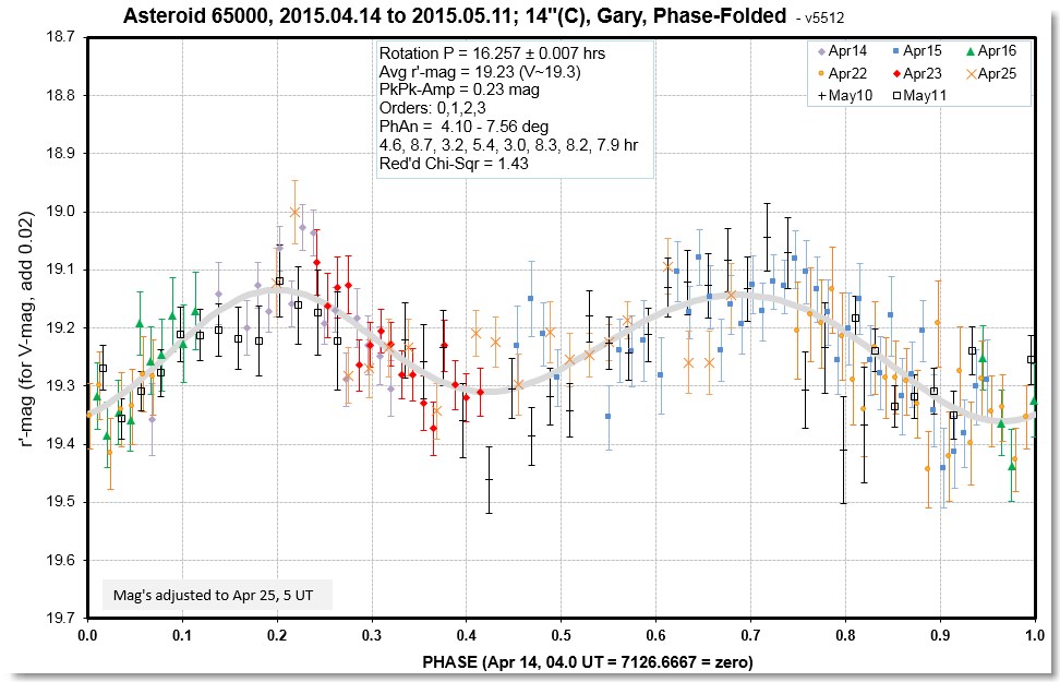
Figure 1a. Phase-folded LC of a Trojan asteroid made with
a 14" telescope from typical observing sessions on 8
dates. Each data point is an average of the magnitude readings
from 9 images. All images were "star subtracted" (explained in the
text). The median SE for these data is 0.057 mag.
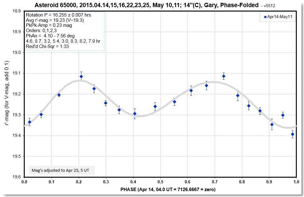
Figure 1b. Same data, but averaged in groups of 10. The
median SE for these averaged data is 0.018 mag.
Many amateurs use the commercial program
Canopus for image processing and light curve (LC) generation.
Canopus was developed by Brian Warner, one of the most experienced
and prolific asteroid observers who ranks higher than his official
status of amateur (he was the first recipient of the Chambliss
Award given by the American Astronomical Association in 2006 for
his extensive contributions to asteroid observing,
characterization, publication and archiving). Canopus is good for
many things, especially bright asteroids, and those with
well-established orbits, but to make use of some of the techniques
that I employ it is necessary to rely upon MaxIm DL for image
analysis and photometry readings plus specially designed Excel
spreadsheets for calibration and LC generation.
Hardware
I refer to my observatory as HAO, for Hereford Arizona
Observatory. The HAO is in Hereford, AZ, which is 90 miles SSE of
Tucson, at a dark site near the border with Mexico, at an altitude
of 4656 feet. I has a MPC site code of G95. A 14" Meade LX200GPS
telescope (vintage 2006) is located in an 8-foot diameter
ExploraDome in my backyard. Everything is controlled from my house
via 100-foot cables in buried conduit. A more detailed description
of my observatory is given at
http://www.brucegary.net/HAO/.
Until very recently I autoguided using the 2nd chip in SBIG CCD
cameras. The main problem with this arrangement is that the
autoguider chip is small, and there are sometimes only faint stars
within its small FOV. Autoguiding quality suffers when using faint
stars, and poor autoguiding leads to increased
point-spread-function (PSF) size and oblong shapes, which
translate to reduced limiting magnitude and the inability to
observe faint asteroids. The prime focus HyperStar configuration
helped in this regard, since the autoguider's FOV was larger, but
the penalty was an image scale that caused main chip PSF to be
defined by image scale instead of the atmosphere. The HyperStar
produces good quality images, but with an image scale of 1.95
"arc/pixel the PSF FWHM was never smaller than ~ 5 "arc. Limiting
magnitude is related to PSF size that has large payoffs for small
PSFs, as shown by the following equation for limiting magnitude
(for a CCD with ~80% QE maximum):
LM = 15.1 + 2.5 * LOG ((D^2 / PSF) + 1.25 * LOG
(g/60s)
where D is telescope effective diameter [inches], PSF is FWHM
["arc], and g = exposure time [sec]. Limiting magnitude, LM, is
defined for SNR = 3 when the photometry aperture radius [pixels]
is twice the PSF's FWHM [pixels]. The importance of small PSF for
limiting magnitude is shown in the next figure.
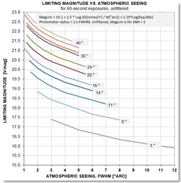
Figure 2. Limiting magnitude vs.PSF size for a selection
of telescope apertures (assumes CCD QE max ~ 80%).
My Meade telescope was PEC trained (in RA)
twice, but ~10% of the untrained 8-minute RA variation is still
present without autoguiding. This imperfect tracking leads to
oblong PSF shapes when exposure times exceed 10 or 15 seconds for
the Cassegrain configuration, even with autoguiding using an SBIG
2nd chip. For the HyperStar configuration the imperfect tracking
wasn't noticeable until exposure times exceeded 30 seconds, even
with autoguiding using the SBIG 2nd chip.
The HyperStar configuration was good for having a large FOV, which
was really important for fast-moving NEAs. But the limiting
magnitude penalty caused by large PSFs, plus the loss of aperture
due to 30% blockage from my large 10-position CFW (color filter
wheel), convinced me to switch back to a Cassegrain configuration.
This switch motivated me to explore a better way to autoguide.
Dean Koenig, owner of Starizona (in Tucson), recommended an
off-axis autoguiding system consisting of a 80 mm, f/5 telescope
and a Starlight Xpress LodeStar X2 CCD. This is what I implemented
in April, 2015.
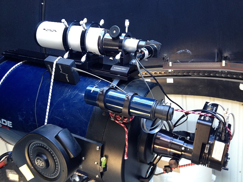
Figure 1. Autoguiding system mounted on a Meade 14"
telescope, consisting of a Orion Short Tube telescope and
Starlight Xpress LodeStar X2 CCD. At the Cassegrain focus
of the Meade 14" is a focuser, SBIG 10-position filter wheel, and
SBIG ST-10XME CCD. The focuser is controlled by a Starizona
MicroTouch wireless focuser.
The autoguiding system has an image scale of
4.3"arc/pixel and a field-of-view (FOV) of 53x42 'arc. Typical
exposure times of 1 second produce autoguiding scatter of ~ 1.0
& 0.7 "arc in the RA/DE axes (Fig. 2). For the main chip of my
SBIG ST-10XME CCD, a typical PSF is ~ 3.2"arc FWHM (it can be as
small as 2.4 "arc), so the atmosphere dominates the PSF size.
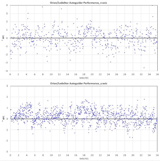
Figure 2. Tracking performance on the first night of
operation of the Orion Short Tube telescope and Starlight Xpress
LodeStar X2 autoguiding system.
The SBIG CCD has an image scale of 0.73 "arc,
unbinned, and a FOV = 27 x 18 'arc. I use 2x2 binning, partly
because the atmospheric PSF does not require 0.73" arc resolution
but also to reduce read noise and download time (from 10 seconds
to ~ 3 seconds). This increases duty cycle, which improves
"information rate" (the bottom line for evaluating any observing
system). Note that even when atmospheric seeing improves to ~ 2.0"
arc, as it does occasionally, there are ~ 3 pixels per FWHM, and
this assures accurate photometry (even for high precision, bright
stars).
For my Meade "mirror flop" is actually "mirror creep" as the
telescope tracks through a large range of hour angles and gravity
loading shifts. With an off-axis autoguiding system this mirror
creep causes the star field to move slowly with respect to the
pixel field. This movement has been measured to be ~ 0.4 'arc/hour
(in RA only). This is small compared with my FOV = 27 x 18 'arc,
and since FOV centering is performed a few times per observing
session, typically, mirror creep is not a problem.
A wireless surveillance camera provides auditory information about
dome and telescope movements, as well as wind sounds.
Observing Procedure
MaxIm DL v5.24 is used for control of the telescope, CCD,
10-position CFW, focuser and dome. A computer is dedicated to
control of the observatory and is not used for any other purpose
in order to not diminish computer resources for this task. The
only exception is a UT/LST clock and TheSkyX for keeping track of
asteroid location.
Exposure times are set to no more than the time required for the
asteroid to move across a PSF's FWHM. For slow moving asteroids
exposure time is limited to 2 minutes. A clear filter is used for
all asteroid observing, except when the asteroid's spectral slope
is desired (when I use g'r'i'z' SDSS filters).
An observing session begins with a manual focus measurement.
The temperature coefficient for focusing is known, so focus checks
are usually not needed for the rest of the night since either
automatic focus changing is turned-on or manual changes are made.
Occasionally a 2nd (or 3rd) focus measurement is made after
cooling stability has been achieved.
Spot checks are made of a chosen star's magnitude to be sure the
dome is synchronized with the telescope pointing, and is not
blocking telescope aperture. Occasional trips to the backyard dome
are also made to assure dome azimuth synchronization.
An observing log is maintained, noting when target observations
begin, filter used, exposure times, focus measurements, dome
changes, visual sightings of clouds, etc.
Approximately once per week I produce a new master flat for any
filter bands that are expected to be used during the next week,
and a new master dark and master bias are produced. My flats are
made shortly after sunset, with a two T-shirt diffuser covering
the aperture. A dark is automatically obtained for each light, and
exposure times are increased to maintain ~ 45,000 counts for the
brightest FOV region.
A computer printout of the asteroid's RA/DE etc for hourly
intervals, obtained from the JPL Horizons web site, is available
for double-checking FOV location. When the asteroid is not easily
seen in any of the images I will copy image files to a flash card
and load them into my main computer for calibration and viewing to
be sure the asteroid is present within the FOV.
Slow moving asteroids will stay within a FOV during an entire
night's observing session. Fast movers may require FOV changes at
1.5-hour intervals. I try to not observe asteroids than move
faster than ~ 900 "arc/hour because they require FOV changes at
intervals shorter than 1.5 hours. If frequent FOV changes are
needed I may go to bed at midnight and set an alarm for whenever a
FOV change is needed. But if FOV changes aren't needed, then I'll
go to bed typically at 1 or 2 AM. I then set an alarm for sometime
before sunrise to manually stop imaging. (I know, I should use CCD
Commander or CCD Autopilot to do this, and one of these days I
will!).
Image Reduction
Procedure
Processing images for each FOV requires about 1.5 hours. My main
computer's RAM (8 GB) will allow ~ 500 images to be loaded by
MaxIm DL without invoking virtual RAM from the hard disk (with a
serious penalty for processing time). This is one reason to use
2x2 binned images, because 1x1 images are 4 times larger and I can
load only ~ 150 of these images at a time for processing. MaxIm DL
(MDL) version 6.x is supposed to overcome this limitation, but it
has some user-unfriendly "upgrades" that I dislike.
All images that have been loaded into MDL are calibrated using
master dark, bias and flat. If necessary, all images are subjected
to a hot pixel removal (typically 30%). Then all images are
star-aligned, usually using just one star near the FOV center.
Automatic star alignment sometimes is inadequate, especially when
a saturated star is in any of the images. My polar axis is aligned
very accurately, so image rotation is never noticeable.
Poor quality images are deleted. The star-aligned images are saved
to a folder. All images are then median combined to produce a FOV
master images. This image is solved using MDL's PinPoint and
saved. It is then subtracted from all individual images to produce
what I call "star subtracted" images. These are saved to another
folder.
The entire process of star subtraction adds an extra 4 minutes to
each FOV's processing time. For faint asteroids, or any asteroids
in a crowded star field, the 4 minutes of extra work is very
worthwhile. In almost every case the benefits for star subtraction
are evident, and this is one reason I can achieve useable LCs for
faint asteroids. I therefore highly recommend use of star
subtraction. (More info on my star subtraction process is given at
http://www.brucegary.net/NEA/StarSubtraction/index.html).
I add an "artificial star" to all of the star subtracted images
(using a DLL created for me by Ajai Sehgal, to whom I shall be
forever indebted). This star is located in the upper-left corner
of each image, and it has the same total flux for every image.
This provides a way to keep track of atmospheric extinction
losses, due to cirrus clouds for example. It is not needed when
using MDL v6, but is is needed for all earlier versions of MDL
because they record photometry files consisting of only magnitudes
(not fluxes, or "intensities" - as MDL refers to them). (More info
on my use of the artificial star is given at
http://brucegary.net/XO1/ArtificialStarPhotometry.htm).
The MDL photometry tool is then invoked. Recall, we are still
working with the star subtracted images. Set the photometry signal
aperture to ~ 1.5 times the FWHM [pixel value], and set the gap
and sky background annulus to 12 pixels each. Assuming the
asteroid can be seen in at least one of the early images, and one
of the late images, it can be specified as a "moving object." (If
the asteroid can't be seen in some images, don't use the "snap to
centroid" feature; just be careful with positioning the photometry
circle for the early and late images where the asteroid can be
seen). When the asteroid can't be seen in any images, other tricks
are possible, but they won't be described here. For 19.2
magnitude, slow-moving asteroids, the asteroid can be easily seen
in every image (with SNR => 5). Specify the artificial star to
be the Reference star. Save the photometry results CSV-file for
later use by Excel.
Load the un-star-subtracted images, add the artificial star, and
invoke the photometry tool again. Specify the "moving object"
again, using the same precautions mentioned above. Specify the
artificial star to be the Reference star. Now, we have lots of
stars in all images, and can choose a couple or 3 dozen of them to
be "Check Stars." Check Star photometry readings have zero effect
on the real-time LC MDL displays; their mag's are just included in
the CSV-file for later use (by Excel). After specifying 20 or 30
stars as "Check" save the CSV-file.
Over the years I've developed an Excel file
that I use as a template for all LC analyses. The first "page" is
a list of targets (RA/DE, mags and transit parameters for
exoplanet stars). A cell is used to indicate which target is to be
processed. The 2nd page is where I import CSV-files. One area is
for importing the CSV-files that include many check stars, and
another section is where I import CSV-files that have only the
star-subtraction readings (their rows are synchronized).
The 3rd page is where I copy mag data from the first page with the
intent that all subsequent pages use those data. So I copy the
mag's with all the check star mag's (from page 2) to this page.
Then I copy the column of star-subtracted mag's to this page,
replacing those that came from the image set with all stars
present. Invariably, a plot shows that the target mag's from the
star-subtracted photometry have "better behavior" than the target
mag's where background stars could cause negative and positive
artifacts to the asteroid's mag readings. Columns of this page
calculate air mass, and also converts each check star's mag to
flux, and creates a column for total check star flux and
corresponding mag. (Of course, this page has the observer's
latitude and longitude).
The next page uses mag's from the previous page 3 user adjusted
cells for achievinge an extinction "fit" to the total flux mag's
from the previous page. A graph of total mag versus air airmass
for guidance.
The next page is complicated because it identifies which check
stars are well behaved and therefore recommended for inclusion for
use in correcting for extinction variations vs. UT. It has a row
of numbers with associated slide bars for incrementing or
decrementing the numbers; when the number for a specific check
star is odd it is included in a total extinction correction; when
it is even it is excluded. The user has feedback cells showing how
the LC fit is affected (and yes, I'm getting ahead of things
here).
The next page is where extinction variations from the previous
page are applied to the target to show what the target's mag would
be if it was above the atmosphere (air mass zero) and there were
no extinction variations. RMS noise is calculated here using
neighbor differences. Many other quality check parameters are
displayed. For example, the user is invited to specify whether
data is accepted or not based on total extinction departure from
the model fit (i.e., "extra losses," due, for example, to cirrus
clouds). The user may also specify a criterion for when data is
too noisy for inclusion.
The next page is unimportant, as it is used to review the LC for
all check stars to look for EBs, transiting exoplanets, or
misbehaving variations among the check stars).
The next page shows the target's LC (e.g., Fig. 1). A model fit
can be determined by adjusting a dozen or more parameters. When
the target is an exoplanet, for example, the user can play with
transit depth, ingress and egress times, transit shape and many
more parameters. When the target is an asteroid the user may
specify a sinusoidal variation superimposed on an average level
(where period, amplitude and phase can be specified). Provision is
made for a slope (linear change of target magnitude with UT) and
"air mass curvature" (caused by the target having an unusual
color, differennt from the check stars chosen to be used as
reference stars). Much of this is described in greater detail in
my book
Exoplanet Observing for Amateurs:
link.
The next page is where chi-square is calculated for the model
specified in the previous page. The chi-square result can be used
in the previous page for automatic parameter solution solving
(using Excel's Solver tool).
The next page is where mag calibration occurs. (It is actually
dealt with before the previous two Excel pages.) Every check star
is a potential calibrator if it has APASS mag's (in the UCAC4
catalog, which contains DR6 mags). I go offline (shell out of
Excel) to run the program C2A:
link.
C2A is a wonderful planetarium program, free, for getting APASS
mags and creating a CSV-file of them for import to Excel. TheSkyX
can also show APASS mag's, but I don't think you can export them
to a CVS-file. With C2A you center the FOV and set the scale to
show all of the FOV, and then export all APASS mag's to a
CVS-file. This file is imported to the Excel calibration page.
Columns are reserved for the check stars, and the user has to
enter a star ID number in a cell. A search of the APASS mag
section then fills cells below the ID number with BVg'r'i' mag's.
Tentative mag's from several pages back are compared with the
APASS mags, and an offset and slope fit can be determined.
Figure 3 shows a plot of "APASS r' minus instrumental mag" vs.
star color (g'-r' - 0.45).
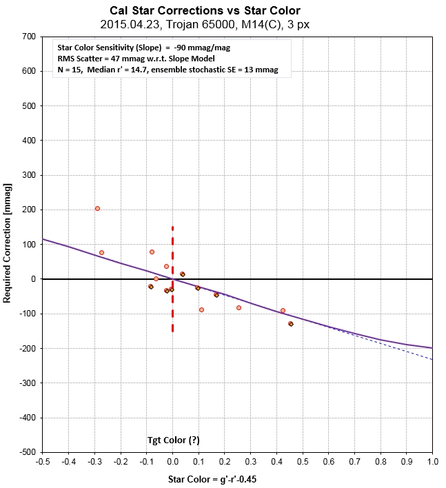 Figure 3. Star color sensitivity plot for one observing
session, using 15 stars with APASS g'r' magnitudes used for
achieving a "CCD transformation" calibration, leading to r'
magnitudes even though a clear filter was used.
Figure 3. Star color sensitivity plot for one observing
session, using 15 stars with APASS g'r' magnitudes used for
achieving a "CCD transformation" calibration, leading to r'
magnitudes even though a clear filter was used.
In this plot a sloped line (with an optional quadratic term) is
fit to the measure mag differences. In this case the slope is -90
mmag/mag. This corresponds to one of the "transformation
coefficients" in the horribly ill-conceived "CCD transformation
equations" that old fashioned astronomers probably still use. For
more information than any sane person wants about the derivation
of CCD Equations, I refer you to:
link.
On that page I explain why CCD Equations were OK when everyone
used log tables instead of calculators, or Marchand calculators
before computers, and why they are totally cumbersome and
unnecessary in today's age of computers with spreadsheets. Having
a display like this is useful in identifying "outlier" stars.
These are stars that vary slowly and weren't identified by the
APASS project as variable, so their mag's at the time of a few
measurements were included in the APASS catalog. But this is years
later, and some of those stars in the APASS catalog have mag's
that are totally different. (Incidentally, CCD Transformation
equations don't allow for this!) I estimate that about 3 to 5% of
all stars are variable at the 20 mmag level (and vary slow enough
to have not been identified as variable by APASS), and therefore
can't be used when 10 mmag accuracy is needed (which is the case
for asteroid work).
Inspection of the above figure shows one star that appears to be
an outlier (upper-left). Indeed, when I use an equation that
compares it's departure from the fitted line with the SE of all
data it is shown to have a <5% probability of "belonging." An
additional check can be made of the 15 APASS stars using a
color/color scatter plot (next figure).
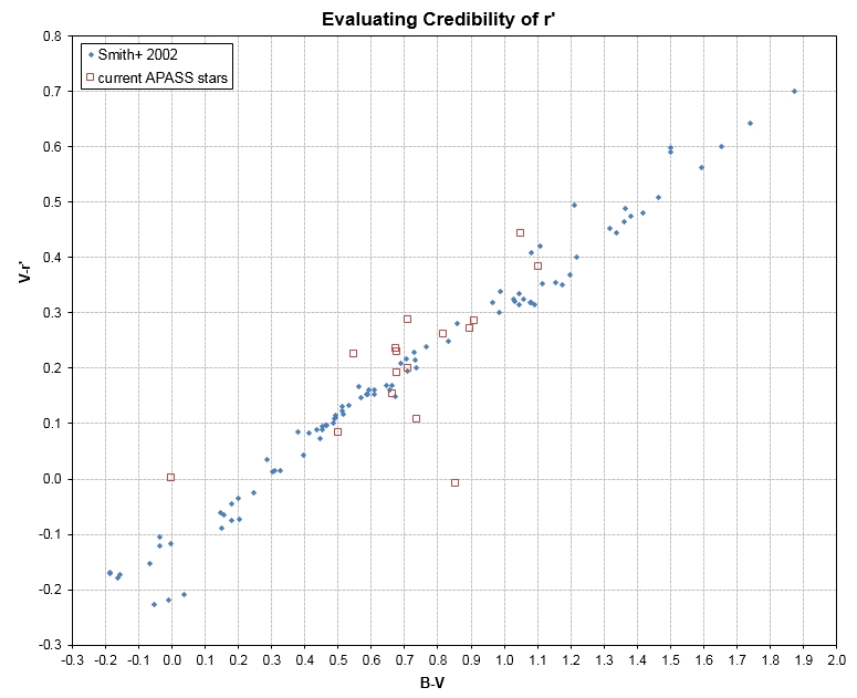 Figure 4. Star color/color scatter diagram showing the
15 APASS candidate reference stars (open red squares) and a set
of ~100 well-calibrated stars (SMith et al, 2002).
Figure 4. Star color/color scatter diagram showing the
15 APASS candidate reference stars (open red squares) and a set
of ~100 well-calibrated stars (SMith et al, 2002).
One of the stars in this scatter plot appears to be an
outlier, and indeed it is the same one identified in the previous
figure as an outlier. I therefore reject it from use (by changing
a cell for it from 1 to 0), and this leads to the following plot.
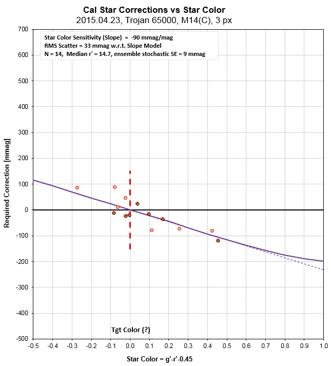
Figure 5. Revised star color sensitivity plot with an
outlier candidate reference star removed.
In Fig. 5 it can be seen that the check star
data exhibit a scatter about the model fit that is 0.032 mag.
There are 14 check stars with useable APASS mag's, so the ensemble
calibration SE is 0.009 mag. There is rarely an occasion when the
ensemble SE exceeds 0.015 mag.
One Fig. 5 subtlety should be mentioned. In this plot I've assumed
the target asteroid has a g'-r'-0.45 color of zero, which is the
sun's color (note: the constant -0.45 was chosen so that the
x-axis is star color difference with respect to the sun). When
there's no information about the asteroid I adopt g'-r'-0.45 =
0.15, which is typical for asteroids. In this case I know that the
asteroid's color is the same as the sun (described later), so I
set the target color to zero (using the above definition for
color).
You might wonder why so much attention is given to achieving an
accurate calibration since we just want to know how the asteroid
varies in brightness as it rotates. The reason we need a good mag
calibration is because almost all asteroids will require
observations with different FOV placements, or on different dates,
and LC segments have to be compared with correct offsets in order
to produce a multi-FOV rotation LC.
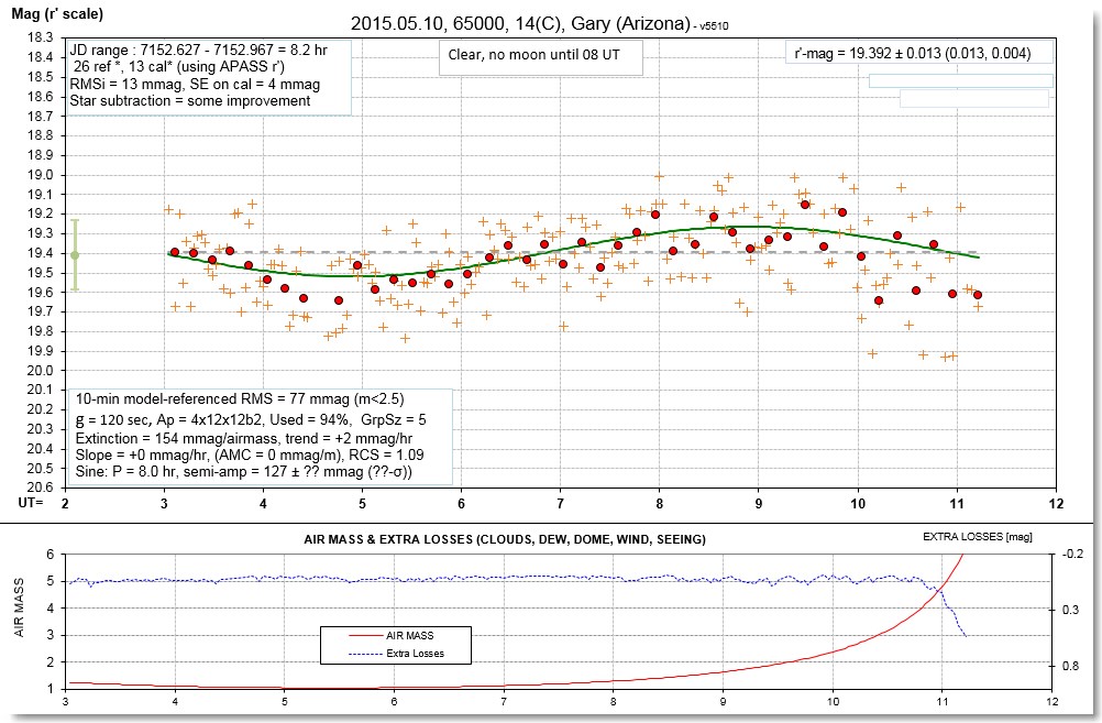
Figure 6. Example light curve for one observing session
(details in the text).
Figure 6 shows a LC segment for one FOV for
the 19.4 mag Trojan asteroid 65000 (depicted in Fig. 1), made on
one of the 8 dates on which it has been observed. The information
box in the upper-left corner shows the JD range of this FOV's
observations (with 2450000 subtracted). It shows that 26
check stars were chosen for use as "reference stars" and 13 stars
were used for calibration (similar to Fig 3). The term "reference
star" needs explanation. A few percent of stars with APASS mags
are slow variables, and they can't be used for calibration but
they can be used to monitor variations due to extinction and
cirrus cloud "extra losses" (because during an observing session
they don't vary). Among those 13 stars used for calibration their
RMS about a star-color-sensitivity slope fit was 13 mmag, and the
ensemble calibration is expected to be accurate to 4 mmag
(assuming APASS mag's are perfect). A comment is given providing a
subjective assessment of how much benefit was afforded by the use
of star-subtraction. Faint asteroids typically benefit the most
from star-subtraction, and asteroids near the Milky Way always
benefit from star-subtraction.
Figure 6 also shows information (lower-left box) about the model
fit. I like using 10-minute RMS as a measure for describing
precision, which is based on the fact that for exoplanet transit
LCs this is an acceptable averaging interval for evaluating
transit depth and shape. For this LC the 10-minute RMS was 77 mmag
(including data for air mass < 2.5). Exposure time for the
individual images was 120 seconds (the small crosses correspond to
individual images). The MDL photometry aperture parameters were 4,
12 and 12 pixels (signal aperture radius = 4 pixels, gap = 12
pixels, sky background annulus = 12 pixels). All images were taken
with 2x2 binning (hence "b2"). 94% of the data were included (some
outliers were rejected from use). The filled circles are averages
of 5 individual image magnitudes. A model extinction of 154
mmag/air mass was used, with a temporal trend of +2 mmag/hour. No
slope was used in the model fitting, and no air mass curvature was
used. The reduced chi-square for the model fit is 1.09. A
sinusoidal variation was used for estimating rgw 10-minute RMS
performance, and it had an adopted period of 8.0 hours and
semi-amplitude of 127 mmag. This sinusoidal model is not used for
any subsequent analysis.
The lower panel shows air mass vs. UT (red trace) and "extra
losses" (blue trace) that departed from the extinction model (that
incorporated a linear trend). Extra losses are usually due to
cirrus clouds, but may occur if the dome is not synchronized with
the telescope. The "extra losses" change starting at ~ 10.7 UT,
when air mass ~ 4 , or EL ~ 14.5 degrees, may be due to the dome
beginning to obstruct the telescope aperture.
Returning to the 10-minute RMS value of 77 mmag, noted in the
lower-left information box, we may convert this to the RMS for
individual images by noting that the exposure time is 2 minutes.
Considering that the download time is 5 seconds, and another 5
seconds is needed for synchronizing with the autoguider, the
cadence is one image per 2.17 minutes. Therefore, within 10
minutes there are 4.6 images, so each image must exhibit an RMS
scatter of 165 mmag (i.e., 0.165 mag). It is commonly thought that
LC quality is limited by the uncertatinty of each image's
magnitude uncertainty; this is true only because the SE per image
determines how averaging of images reduces SE per average of
images. For example, in Fig. 1b the median SE for averages of 90
images is 0.018 mag (this is to be expected since 0.165/sqrt(90) =
0.017).
This completes analysis for an individual FOV. Next we consider
how to combine LC segments from many FOVs, taken at different
times of an observing session, or on different dates. The first
matter to consider is that an asteroid is continually changing
brightness even if it doesn't rotate, due to changing distances (r
and d) and changing viewing geometry (phase angle). I use the JPL
Horizons ephemeris as a guide in correcting measured magnitude for
a given JD to what it is expected to have at a standard JD
(usually chosen to be the first JD of the first FOV for that
asteroid). The next figure shows JPL Horizons predicted ephemeris
magnitude vs. time for the Trojan 65000 observations during the 4
weeks of observations.
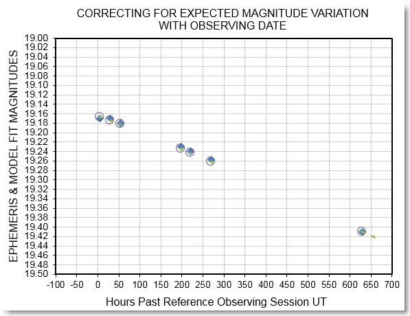
Figure 7. Ephemeris magnitude vs. observing date and
3rd-order model fit. Solid blue diamonds are the ephemeris
values, circles are the fitted values and small green symbols
represent values for offsetting observations.
The ephemeris data were fitted by a polynomial which was then used
for offsetting measured magnitudes to a standard date 0 hours)
before phase-folding analysis is performed.
Figure 8. Phase-folded LC for observations on 8
dates during a 4 week period (same as Fig. 1). Each data point is
an average of magnitude readings from 9 images. Using chi-square
> 10 as a guide outlier data were identified (8 out of 186
images) and excluded from the fitting process.
The phase-folded LC, above, is based on 286
images, all subjected to the star-subtraction process, with a 96%
acceptance using chi-square > 10 as a rejection criterion. A
3-term harmonic sinusoidal fit was performed using a fundamental
frequency (corresponding to 1/2 the rotation period) and two
others (corresponding to the rotation period and 1/4th the
rotation period). Free parameter status was given to the amplitude
and phase for each sinusoid, as well as the period of the
fundamental and an offset.
After a solution was found, free parameter status was given to an
offset for each observing session, normalized by 0.020 mag, an
estimate of maximum "observing session offset" due to calibration
uncertainties. This was done because such offsets are expected to
exist.due to an imperfect calibration using a finite number of
APASS stars for each observing session (as well as imperfect
ephemeris magnitude changes with date due to the use of a default
phase effect, using G = 0.15). The "observing offsets" increased
with phase angle in a way that implies the need for a larger G
(i.e., G = 0.30). The RMS difference between "observing session
offset" and a model with a better G value is 0.023 mag. This is
considered acceptable. After the "observing session offsets" were
solved for another iteration of the phase-folded magnitudes is
performed.
The information box in Fig. 8 states that "Red'd Chi-Sqr = 1.43"
which means that either another component of variation is present
in the data that has not been modeled or my estimated SE values
are slightly optimistic (by 20%). If this asteroid was a binary
then the smaller component could produce another variation with a
period corresponding to that component's rotation period, which
isn't necessarily the same as the primary's rotation period. It is
therefore worth checking to see if the "residuals" off the above
phase-folded LC exhibit a variation that can be fit by another
sinusoidal model.
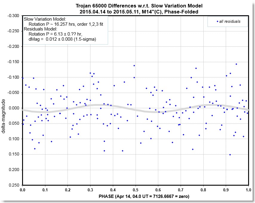
Figure 9. Phase-fold fitting of residuals off the model
in Fig. 6 showing that there is no significant variation in
addition to the one in the Fig. 6 model.
As this graph shows the Fig. 8 residuals do not exhibit a
statistically significant variation. Therefore, we have no evidence
for a second component contributing to brightness variability for
this asteroid. We therefore should investigate the possibility that
a higher order sinusoidal harmonic fit is required.
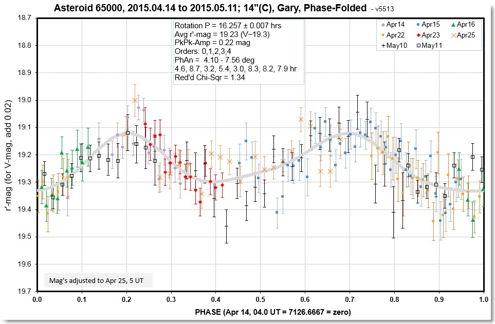
Figure 8. This is a 4th-order fit (4th harmonic of the
fundamental), providing a slightly better fit to the data.
This slightly better fit now includes 98% of
data as acceptable (4 rejected out of 186), using a chi-square
criterion of 10. However, it still has a reduced chi-square
greater than one (1.34), and I don't think the data deserves any
more higher order terms for the model. What's normally done in
this situation is to arbitrarily increase the SE estimates (all of
them) by the suggested 16% and repeat the chi-square fitting. This
isn't necessary in this situation because we would just arrive at
the same solution and the only difference would be a slightly
greater SE for the model parameters that are solved for. There is
negligible effect on the period; the solution SE for P has an
uncertainty that is still 0.007 hrs.
Asteroid
Feasibility Regions
The "exercise" above illustrates the feasibility of observing a
19.3 magnitude asteroid with a 14" telescope, provided the
asteroid moves slow enough that long exposure times are possible.
The observations in the example were made with 2-minute exposure
times, and the the PSF FWHM was typically 3.2 "arc. In order for
the crossing time for this PSF to be less than 2 minutes the
asteroid motion must be < 100 "arc/hour. This should include
all Trojan asteroids, for example, and most main belt asteroids.
The fast movers will be NEAs. The following diagram is a plot of
magnitude versus rate of motion showing "observability" for
various telescope systems.
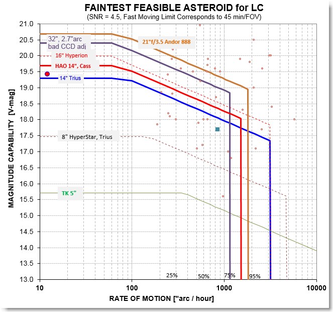
Figure 11. "Feasibility" diagram for
asteroids, showing area within which observations are feasible
for various telescopes (when the sky is dark). The red dot
corresponds to Trojan 65000 (on 2015 May 11), a slow mover. The
green square is typical of a Near Earth Asteroid (NEA), with a
typical rate of motion of typically ~850 "arc/hour. The %
numbers at the bottom show what percentage of NEAs are moving
slower than their rate of motion location. More details are
described in the text.
This graph is useful in quickly determining if an asteroid can be
observed with a specific telescope system. For example, the Trojan
65000 used for this case study was moving at ~ 20 "arc/hour and was
at V-mag ~ 19.4 on the last day I observed it. This is shown by the
red dot, and it is "within" the feasibility region for the
telesccope system labeled "HAO 14", Cass." A typical NEA might be at
the location indicated by the green square, at 850 "arc/hour and
V-mag = 17.7. It too would be observable by my 14" telescope. But a
NEA moving at the same rate that is fainter than ~ 18.4 would be too
faint for my telescope. If 20th magnitude is desired then a Hyperion
16" would be acceptable, for example.
This graph assumes that the asteroid must register in most images
with a SNR > 4.5 in order to be capable of producing a useable
LC. With my 14" I can "see" 20.0 stars when the sky is dark, images
are sharp and exposure times are 2 minutes; so that's a limiting
magnitude for 2-minute exposures (for the standard 60 second
exposures subtract 0.4 mag, yielding a standard limiting magnitude
of 19.6 for my telescope).
Moonlight can reduce limiting magnitude by about 1 magnitude (full
moon, 45 degrees away), so that should be taken into account when
using the feasibility graph.
CCD QE is also a factor in limiting magnitude. The above feasibility
graph assumes 80% QE, which corresponds to my SBIG ST-10XME
(KAF-3200E chip).
Links:
HAO
description
Master
list of B.Gary web pages
B.Gary resume
________________________________________________________________
This site opened: 2015.04.20. by Bruce L.
Gary (B L G A R Y at u m i c
h dot e d u). Last
updated: 2016.04.06