Whereas most amateurs use a differential photometry procedure to measure an unknown star's brightness, and professionals use a "pipeline" linkage of programs to perform PSF-fitting, etc to accomplish the same task, I prefer to use an "artificial star" photometry procedure. I don't know if anyone else does it this way, so in this web page I'll describe it in perhaps too much detail.
My philosophy for data analysis is to "be as close to the data as possible." By that I mean that I only resort to automated procedures after I've had sufficient experience with viewing the data in spreadsheets to know what kinds of problems can be present so that the automated procedure can safequard against being misled by bad data. For example, clouds not only make photometric results noisier but they may also prodcuce biases. Neither effect is desireable, so any analysis procedure must explicitly reject cloud-contaminated data before creating a transit light curve.
Another of my data analysis philosophies is to "always be on the lookout for trouble." If something doesn't seem right, or something is noticed that can't be explained, STOP and figure it out before proceeding! This practice has saved me many wasted hours when I worked with data before retirement, and I believe it is a good philosophy with all types of data.
I like spreadsheets for the "learning phase" of any data analysis procedure. I consider myself to be still learning to do photometry, so as I flounder I like to see graphs of things in order to at least confirm what I expect if not to notice things I don't expect. Therefore, in what follows you will notice that the bulk of work is done with Excel spreadsheets.
The following analysis is designed to identify bad images so that they're not used in producing a transit light curve. An image can be "bad" because a cloud passed through the line of sight during the exposure, or the wind caused bad tracking (with an oblong shape for all star images), or a downslope wind caused star field movement that was too fast for the tip/tilt image stabilizer (the SBIG AO-7) to follow. This last problem is common at my site. The downslope winds also can produce a 'ballooning" of seeing that can last a few seconds, which I assume is caused by the breakdown of Kelvin-Helmholtz waves at the top of the downslope wind plume (at the interface with ambient air). Rejecting "bad" images can be important in rescuing what would otherwise be a useless observing session.
Preparing CVS-Files for Importing to Excel
Identifying a "bad" image is accomplished by comparing the measured flux of a bright, unsaturated star (the same one for all images for that night) with the flux of an artifical star that is placed in the upper-left corner of each image before photometry readings are made. I refer to the bright star as my "extinction star" for the night, for reasons that will be obvious shortly. The next few paragraphs are detailed enough that anyone using MaxIm DL (MDL) will be able to reproduce my procedure, and anyone using a different image analysis program should be able to follow the concepts and translate them to the other program's requirements.
A group of ~30 images are loaded into MDL. They are subjected to a "Calibrate All" command which applies a dark frame subtraction and flat frame division. Next I create an artificial star in the upper-left corner of each image using Ajai Sehgal's plug-in (that replaces a 64x64 pixel region with a star having a Gaussian shape). This takes a few seconds, and here's what an image with the artifical star looks like.
Figure 1. An artifical star has been placed in the upper-left corner of this calibrated image, making it ready for photometry.
Next I use the MDL Photometry Tool to batch process the group of 30 images in a way that allows the flux for a chosen bright star to be related to the flux of the artifical star (always the same, 1,334,130 counts). The same bright star has to be used for all images taken during an observing session. [The rest of this paragraph and the next one are tedious, so feel free to skip them; they're just a "how to" if you're using MDL.] The specific procedure using MDL, once a group of 30 images have the artifical star, is to click Analyze/Photometry, verify that the boxes for "Act on all images", "Use star matching" and "Snap to centroid" are all checked, select "New Object" (from the Mouse click tags pull-down menu), click on the bright (unsaturated) star to be used for monitoring extinction for the observing session, select "New reference star" from the pull-down menu, and click on the artificial star. Then click on "View Plot" (which displays a plot of the magnitude of the extinction star relative to the artifical star, taken to be zero). Save this photometry solution to a CSV-file ("comma-separated-variable). The CSV-file is automatically placed in the directory "My Data Sources." As soon as this CSV-file exists, open Excel and import the CSV-file data to a cell. (Of course I use a worksheet template with many other cells ready for later analyses; this concept will be obvious to any spreadsheet user). Excel's data importing defaults to the CSV-file just created, so with that file highlighted simply depress the Enter key. Complete the import using Alt-N, Alt-C, Alt-F, Enter. The spreadsheet now has 3 columns: JD, the objects magnitde relative to the artificccial star, and zero (for the artificial star's magnitude relative to itself).
If the above paragraph's procedure were repeated for all remaining groups of images, and if each CSV-file data import is placed below the preceding one, an analysis could be performed for deriving extinction for the observing session and identifying bad images. However, since MDL has calibrated and artificial star modified images in the Photometry Tool work area, it is better to click "Back" on the photometry graphical display and untag the the "Obj1" and "Ref1" selections and proceed to perform pohotometry on the exoplanet star and nearby reference and check stars. Select "New Object" and click on the exoplanet star. Select "New Check Star" and click in a set sequence of stars to be used in the spreadsheet as reference stars and check stars. Finally, Select "New Reference Star" and click the artificial star. View the photometry plot and save the solution to a CSV-file. Switch to the Excel spreadsheet an import this data to the same row but different column as its corresponding extinction star data.
Spreadsheet Extinction Quality Checks
Repeat the operation described in the previous two paragraphs for all groups of 30 or so images. All remaining analyses will be done with the spreadsheet. An example of what's been described is shown in the next figure.
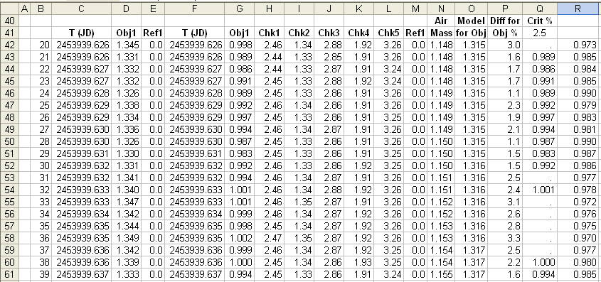
Figure 2. Photometry relative to an artificial star is shown after importing CSV files to an Excel spreadsheet. Each row is for an image (images numbers 20 through 39 are shown). Column D is the "extinction star" magnitude realtive to the artificial star, column G is the same for the exoplanet candidate and columns H through L are for stars that will be used in the spreadsheet as reference or check stars. Column N is air mass (calculated from image number, using a LS solution). Column O is a prediction for column D data based on an extinction model (where the user adjusts a zenith extinction to achieve a good fit, see below). Column P is a percent difference of column D with respect to column O (i.e., this column is a percent discrepancy between measured extinction star flux and extinction model flux). Column Q is a repeat of column G when the absolute value of column P is less than the criterion in cell Q41 (2.5%). The last column is the deduced additional extinction caused by clouds (or flus loss due to bad tracking, bad seeing, etc).
Yes, this is a lot of work, and it's done in a spreadsheet. Normally, differential photometry is done by specifying reference stars and their magnitudes when the Photometry Tool is invoked. I prefer to do as much analysis as possible in a spreadsheet, where bad data can be easily identified rejected. This will become clearer in the next few paragraphs.
In the previous figure notice that we have image quality information for each image. By adjusting the value for zenith extinction in a cell we can determine whether clouds were present and how much additional extinction they contributed, image by image. This is shown in the next figure.
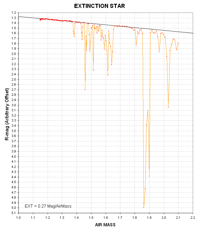
Figure 3. Plot of magnitude difference of the "extinction star" relative to the artificial star versus air mass. The straight line is for a zenith extinction determiend to be 0.27 magnitude per air mass.
This figure is for an observing session that started out near the meridian when it was clear and gradually clouds moved in producing at their worst ~4 magnitudes of additional extinction. The next figure shows the "transparency" of clouds versus time, which is derived from the difference between total extinction and model extinction.
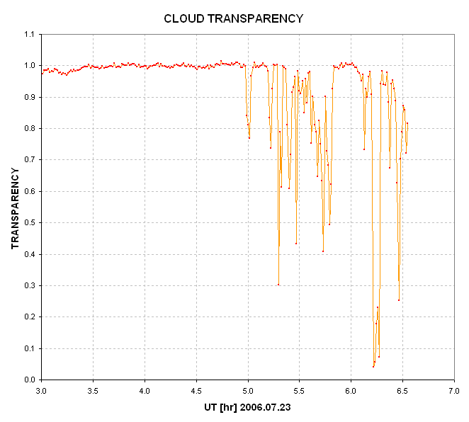
Figure 4. Transparency of clouds during a 4.5-hour observing session, based on comparing a bright star's flux with the artifical star's flux and removing the effect of a normal clear sky extinction.
In this figure all departures from 1.00 are due either to clouds, bad tracking or exceedingly bad seeing. These departures will not affect the artificial star but will reduce the flux from a chosen "extinction star." Visual inspection of the images show that for this observing session there were no tracking errors or no seeing degradations (FWHM = 2.6 to 3.5 "arc). Clear conditions were present from ~3.4 UT to 4.9 UT, and my observing log did indeed show that clouds were present after 4.9 UT.
I have established that by setting an acceptance threshold of ~2.5% all accepted data appear to be useable for establishing an exoplanet light curve.
Using Reference Stars
So far we haven't made use of reference stars (also called "comp" or "comparison" stars - a leftover term from "visual" brightness estimating days). Other columns are used to calculate magnitude shifts that should place all stars on the correct magnitude scale using whichever stars for reference the user wants to try. Consider the next figure.
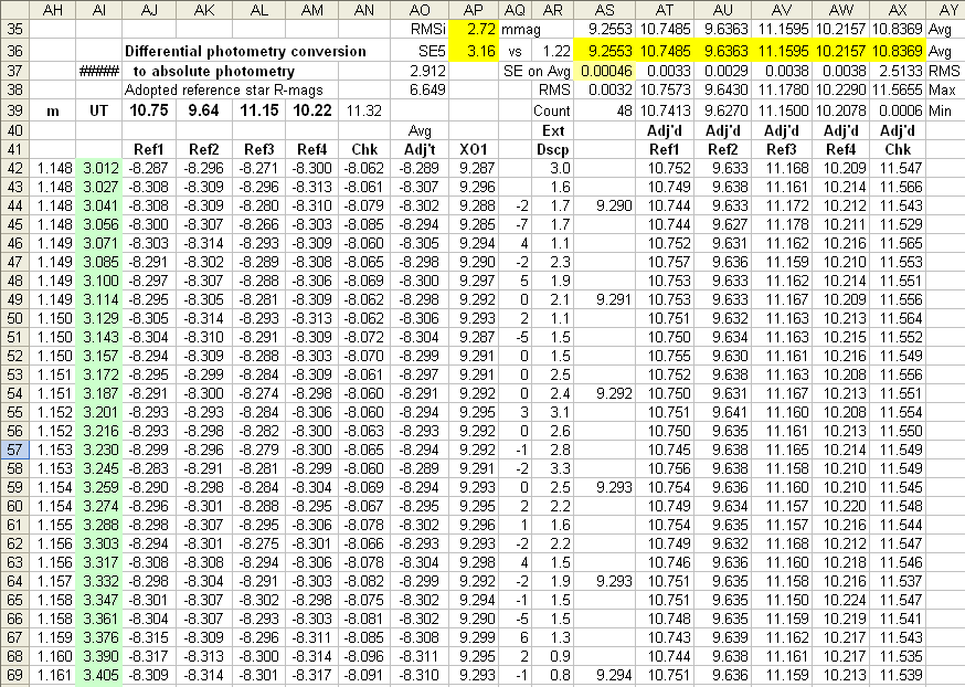
Figure 5. Portion of the same Excel spreadsheet as in Fig. 2, showing where reference stars (columns AJ - AM) are used to calculate a magnitude offset (column AO) that is applied to the exoplanet "instrumental" magnitudes (not shown) to arrive at corrected exoplanet magnitudes (column AP). The same offset magnitudes are applied to the reference and check star "instrumental" magnitudes to arrive at corrected reference star and check star magnitudes (columns AT - AX). Column AR is a repeat of another column where discrepancies are calculated for the "extinction star" and a model (predicted value) for the extinction star (the discrepancy provides a way to identify cloud-contaminated images). Column AQ is a difference of the exoplanet's magnitude for the image associated with its row and the average of its 4 nearest neighbors; this also helps identify outlier images. Column AS is a 5-point average (non-overlapping).
Columns AQ and AR are used to identify outlier data. Whereas the column for additional cloud extinction (AR) is fairly straight-forward, an outlier in column AQ may call for further consideration. A bad tracking image would show up in AQ as an outlier without necessarily showing anomalous extinction. When a row is judged to be unuseable it is "rejected" by deleting the contents of the exoplanet magnitude (column AP).
Another quality check is afforded by plotting corrected reference star and check star magnitudes (columns AT - AX). If any of these stars are variable, or noisy, then additional consideration is called for. On more than one occasion I've had to reject a reference star from use because it didn't behave well in one of these plots. Rejecting a reference star is done simply by chaning which columns are averaged (AJ - AM) to produce column AO. This is very easy, which contrasts with the standard Ensemble Differential Photometry procedure that would require a remeasurment of all images with a different reference star assignment.