Additional PAWM Supporting Material
This web page is a "catch-all" for material
supporting aspects of PAWM that don't have sufficient "general
interest" to appear on the PAWM home page.
Links Internal to This Web Page
Expected Comprehensiveness
of PAWM
Suggestions for Observing,
Data Analysis and Data/LC Submission
TheSky/Six Display of WDs
Defining "Percentage Coverage"
Achieving Completeness With
Short Observing Sessions
Description of Data Files
Comparing Observers
Spurious Sinusoidal Amplitude
Problem (4 regions)
Overlapping LC Result
UCAC3-Based
V-Magnitudes
Debris Disk Animation
Expected
Comprehensiveness of PAWM
The following two figures are repeated
from the PAWM home page.
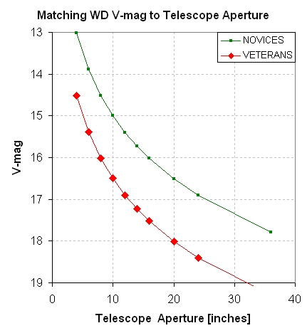
Figure 1 Left: Preliminary result showing
the faintest V-mag's for which useful LCs can be obtained versus
telescope aperture.
Figure 1 Right: The number of known WDs
brighter than V-mag values.
The left panel, above, will be revised as PAWM
observations enter the archive. So far this is a conservative
interpretation of the first two submissions. Combining information
in the two panels leads to the conclusion that a 14-inch telescope
is capable of characterizing more than ~2500 WDs, provided experienced
users are involved.
I was asked "Where does the funtional relationship
for the left panel come from?" It's based on an empirical relationship
for limiting magnitude as a function of CCD exposure time, atmospheric
seeing and telescope aperture, for "novice" and "experienced" users:
Novice Users:
ML = 14.9 + 5 * LOG10 (D [inches])
- 2.5 * LOG10 (W ["arc) + 1.25 * LOG10 (g
[minutes])
(1)
Experienced Users: ML =
15.8 + 5 * LOG10 (D [inches]) - 2.5 * LOG10
(W ["arc) + 1.25 * LOG10 (g [minutes])
(2)
where D is telescope aperture [inches], W is
the PSF's FWHM ["arc] and g is CCD exposure time ("gate time"
for engineers) [minutes]. The constant 14.87 is determined empirically
for use of a SBIG ST-8XE CCD camera and an unfiltered passband. Limiting
magnitude, ML, is defined here as a magnitude for which an "optimized
photometry aperture radius" produces SNR = 3. The term "optimized
photometry radius" needs explanation. When constructing a light curve
(LC) from an image set where "atmospheric seeing" is approximately
constant there is a photometry aperture radius that produces a minimum
in the LC's RMS. The best photometry aperture radius is ~ 2.5 x FWHM
for bright stars; considering ever fainter stars this optimum radius decreases
to ~ 1.0 x FWHM, which is a common choice for asteroids. This range of
values, 2.5 to 1.0, is based on "real world" measurement experience; a
theoretical treatment that neglects such real world issues as variable seeing
predicts a best radius of 0.75 x FWHM for stars of all brightnesses (when
only 65% of the star's flux is captured).
The above equation is for bright stars. Since
WDs range from "bright" to "faint" the constant in the above
equation should vary with WD magnitude. One of the goals for
PAWM is to establish, from WD LCs submitted by many amateur observers
(with different "atmospheric seeing"), an empirical relationship
for the curve in the left panel, above. The final curve is likely to
have a slightly different "slope" because of the dependence of best
photometry size on star brightness.
Suggestions for Observing, Data Analysis and Data/LC Submission
Suggested Observing Procedure
Exposure times should be 30 to 60 seconds,
with 30 seconds preferred for the bright WDs. With an image
download time of ~ 10 seconds the duty cycle for observing
should be acceptable for these exposure times.
I recommend observing either unfiltered,
or with a "clear with blue-blocking" filter (which I refer
to as a Cbb), or an Rc or r'-band filter. Since we won't be observing
close to the horizon there's no need to employ a Ic or i' or z'
filters. There is one situation where these long wavelength filters
may be useful, and that's when the moon is close to a target. Full
moon in September occurs on September 12/13 (when moon's DE =0).
When observers work the same target in coordination it is not necessary
that all use the same filter since we're just looking for a big
transit feature.
Flat field calibration and autoguiding
are perhaps less important when searching for transit depths
of hundreds of mmag, but why not adhere to the good practices
that have served us well for observing known exoplanet stars.
The brighter WDs (V-mag < 14) will have finder
images at the Villanova White Dwarf Catalog (link).
The fainter ones, however, will usually only be identifiable
in your images by performing a PinPoint plate solve on a sharp image
and then searching for a star at the WD's coordinates. I might add
a finder image with the WD identified in a column of the WDtargets
web page (link) for
these faint WDs.
Image Processing Cautions
Since we're searching for a very brief
fade of large amount it is important to disable any outlier
rejection procedures that were created for analyzing main
sequence star exoplanet transits. Any submitted LC or data file
should include ALL data that is accepted based on image properties
(e.g., images with poor autoguiding should be rejected from analysis
prior to producing a light curve).
Selecting reference stars should be
done carefully, which is something I've preached for the
past 3 years. During my exoplanet observing I've encountered
two flare stars and several delta Scuti stars among my reference
candidates, and if a single flare star star is used for reference
it would make the target star look like it underwent a brief and
deep transit; similarly, if a delta Scuti is used for reference the
target star would appear to undergo delta Scuti variations. I normally
include up to 28 stars plus the target star in my photometry measurements
when creating CSV-files for import to a spreadsheet where an optimum
subset of the 28 candidates are used for reference (total star flux,
etc). I visually inspect a LC plot that includes all of the candidate
stars inorder to identify "misbehavior." This is described in my exoplanet
book (Chapter 18).
For faint targets the best photometry
apertures are smaller than for V-mag 10 -13 stars. For
example, I've found that for a 14-inch telescope the optimum
photometry radius is ~ 2.5 x FWHM for V-mag ~ 10 - 13, 1.5 x
FWHM for V-mag ~ 14, and 1.2 x FWHM for fainter targets. Please keep
copies of your image sets in case re-processing them is needed.
Data Submission Procedure
You may attach (or embed) a light curve
plot to an e-mail, or attach a data file with a format the
same as given at this link. I will
maintain links to a web page devoted to each WD that is observed.
The data files have a link below the light curve (for those whowant
to perform additional analyses). The web page "List of hot and cold
WD targets" (link)
will show how many hours of LC observations have been accumulated
for each target, and it will include a link to a web page devoted
to each observed target.
If you submit a light curve plot (jpg preferred)
I suggest that you use a standard magnitude range of 1.0 magnitude
and a standard time interval of 8 hours (unless more are needed). If we
all use the x- and y-axes scale it will be easier to compare LC features
from different observers.
Displaying WDs Using TheSky/Six
Howard Relles provided me with a spreadsheet
of white dwarf information for those with V-mag < 16. In addition
to V-mag the WD B-V color is included (where it exists) and for
some WDs a r'-magnitude is included. From the spreadsheet I created
an ASCII fixed format file for the V-mag ranges <14, 14-15, 15-16
and 16-17. These were compiled by TheSky/Six, which produced 3 sdb-files
that are automatically loaded when I run TheSky/Six. Using the "Display
Explorer" menu I can toggle the display of V-mag or B-V for any of
the 3 WD brightness categories. Here's an example for WDs having V-mag
= 15 - 16 (needs a wide screen to see it all):
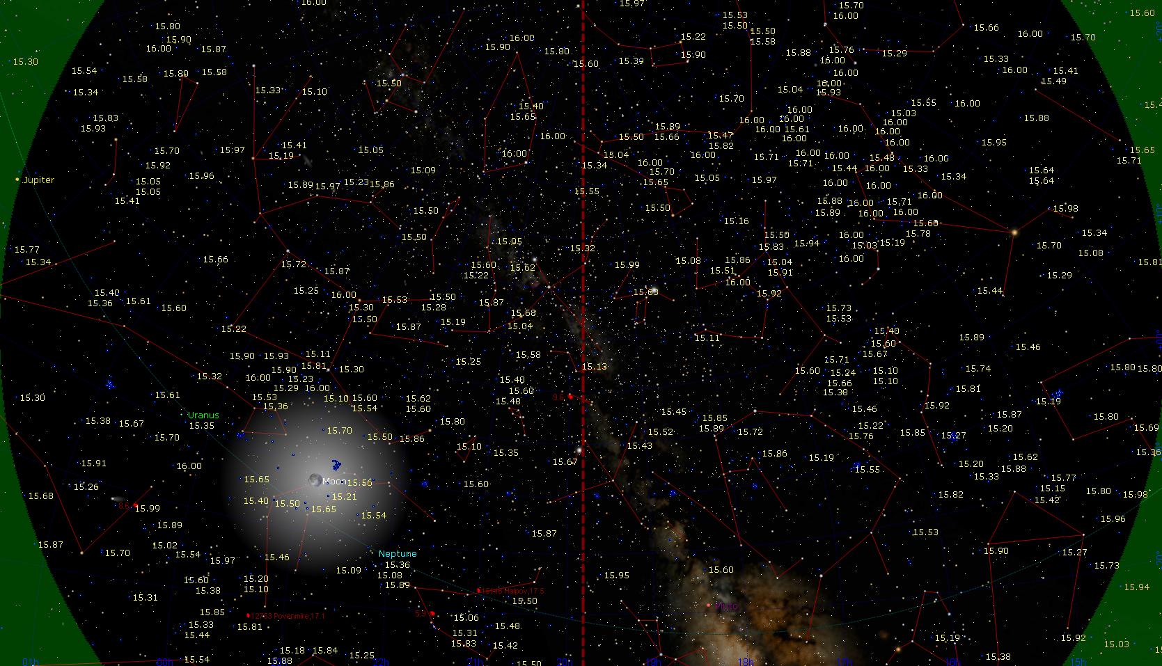
Figure 2. TheSky/Six display for the
HAO observing site at local midnight in late July. Yellow magnitudes
show white dwarf locations and their V-mag value (for V-mag between
15 and 16). By toggling the state of a menu box the B-V colors
for these WDs can be displayed. The same capability is available
for WDs with V-mag < 14, or between 14 and 15.
I'll use displays such as this for producing
WD candidates needing observations.
If anyone wants a copy of the sdb-files you
may e-mail me your request and I'll ask Howard if he's willing
to share them (since his original catalog is proprietory at this
time).
Defining
"Completeness Coverage"
Before a target has been observed it has zero "completeness
coerage" for all periods of interest, P = 4 to 32 hours.
After an 8-hour session its completeness coverage
is 100% for P <= 8 hrs, and lower values for longer P. For
example, completeness coverage for P = 32 hrs is 25%. For 16 hrs
it is 50%, etc.
If another 8-hour observing session is made at a
random time the completeness coverage versus P cannot be calculated
until the relationship between the two 8-hour observing sessions
is specified. A simulation using random start times for 8-hour sessions
is presented in the next section (Fig. 4.). It is constructed by specifying
a set of start times, fixing the end times to 8 hours later, choosing
an arbitrary reference time (such as the beginning of the first observation),
and for each P value (from 4 to 32 hours) calculating whether or not
any of the observing sessions was ngoing during each of 20 phase values
(e.g., phase = 0.025, 0.075, 0.125, etc). Phase is defined zero at the
reference time, and it varies linearly to 1.00 one period later. Every
observing time during an observing session can be assigned a phase value
by subtracting integer periods, as necessary, to arrive at a fractional
period, and this fractional part is the phase. Here's an example of
a "completeness coverage" plot.
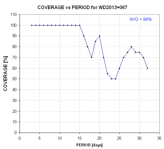
Figure 3. Percentage coverage versus period
for star WD2013+067.
Notice that the completeness coverage trace is not
monotonic. This is because the phase range for one observing session
can mostly overly the phase range for another observing session, for
a specific period, while having less overlap for other periods. For
this plot the average coverage is 84%. I think PAWM will adopt 75%
as a criterion for re-categorizing a target WD from the "hot" list
to the "cold" list.
Achieving
Completeness With Short Observing Sessions
The most desireable observing strategy for WDs
with periods as long as 32 hours is to obtain a set of light curves
that achieve complete coverage for any 32-hour observing interval.
A spacecraft could do this, but mid-latitude ground stations are limited
to ~ 11 hours per observing session during winter. In September (autumnal
equinox) observing sessions are limited to about 10 hours. Consider
the case of even shorter observing sessions, 8 hours, made at randoom
times. How many of these sessions are needed to achieve ~80% coverage
of a 32-hour exoplanet period.
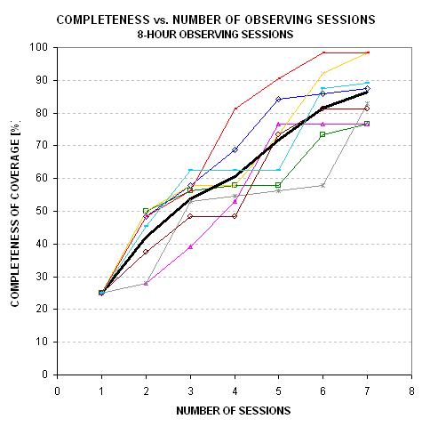
Figure 4. Completeness of coverage of
32-hour period exoplanet using only 8-hour observing sessions
and a Monte Carlo simulation, assuming that observing sessions
are made at random times.
This Monte Carlo simulation shows that on average
80% coverage is achieved after six 8-hour observing sessions.
Description
of Data Files
Data files contain a "header" with information about the UT StartDate,
Object, Observer, etc, followed by data in the form of JD and intrumental
magnitude (using any offset, it doesn't matter). Here's an example of a
header:
StartDate : 20110801
Object : WD1822+410
Observer : Garlitz, Joe (GJP)
E-mail : garlitzj@eoni.com
Country/State : Oregon
Latitude : +45.5728
ELongitude : -117.9208
Aperture : 12-inch
Filter : C
Exposure : 60 sec
ClockCorrn : 0 sec
Comment : 5 ref stars. Clr, no moon, seeing normal.
Comment : Column headings are JD & Instrumental Magnitude
and here's an example of a header followed by data:
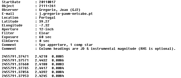
Figure 5. Example of header with data lines, to be attached to an e-mail sent to Bruce Gary at the PAWM e-mail address: 
Note: the data lines have a 3rd column, which in this case is the observer's estimate of RMS. Any data following the first two columns is ignored in my processing.
The JD and magnitude entries may be separated by spaces, commas or tabs. The filename convention is date (YYYYMMDD), target, Observer code, "raw.txt" - with spaces between, as illustrated by the following: raw data filename
20110801 WD1822+410 GJP raw.txt
When an observer sends me a raw data file, I import it to an Excel spreadsheet where it eventually produces a light curve (LC). The LC is fitted by a simple model that allows for a temporal trend and air mass curvature. The temporal trend may be caused by an imperfect flat field and imperfect autoguiding. The air mass curvature is almost always caused by the target star having a different color from the average of the reference stars (or the single comp star if just one reference is used). The model also permits fitting a transit with several free parameters, but for PAWM this feature may never be needed. A screen capture of the LC is placed on the PAWM web page devoted to the target star.
Below each LC graph I (usually) include links to
two data files. The first one is the raw data file sent to me
by the observer. The second one consists of four processed magnitude
types, plus RMS. Here's an example of this data file, with "spo" replacing
"raw" in the orignal filename.
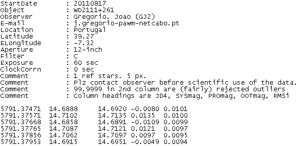
Figure 6. Example of a "spo" data file. The JD format has
been shortened. The 3 mag columns are explained in the text. The last column
is RMS.
The "spo" header comment lines have been slightly modified from the
raw data file header. The JD is in what I call JD4 format. The first magnitude
(2nd column) does not have "systematic effects" removed. Hence, when plotted,
it may have a temporal trend and air mass curvature pattern. These are the
magnitudes I use in plotting the light curves on this PAWM web site. The
second magnitude (3rd column) has systematics removed. I can produce light
curve plots of this data, but none are presented at the PAWM web site. The
third magnitude (4th column) is the same as the previous magnitude except
that an everage has been subtracted. These magniutdes are ideal for plotting
when searchig for similar structure in different LCs, or when performig phase-folding
analyses. The last column is RMS for the JD4 region.
Comparing Observers
It may be useful to compare one's RMS performance with
others after compensating for the observer's telescope aperture and star
brightness. I have done this by standardizing the measured RMS10 to what
could be expected if the same observer had used a 14-inch aperture telescope
while observing a star with V-mag = 14.0. This conversion is "tricky" because,
for example, the level of scintillation changes, yet scintillation typically
contriutes only ~ 1/2 of the total to RMS10.
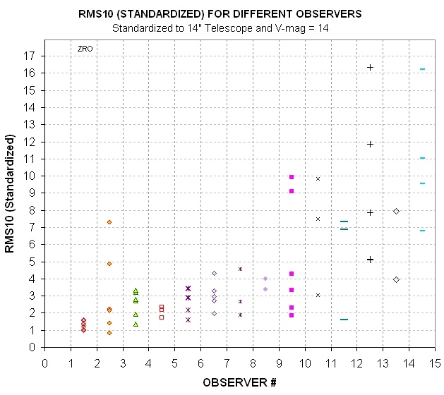
Figure 7. RMS10 standardized to a 14-inch
telescope and V-mag = 14.0, for various observers. The best observers by
this measure is Roberto Zambelli (Italy), who uses a 10-inch telescope and
a G-band 495 nm long-pass Baader filter.
I define "RMS10 Standardized" = (RMS10meas'd - 0.5 mmag)
* (Aperture/14")2 * 2.512 (14-V) * (1 + (Aperture/14)0.67)/2
The above equation assumes that there's a "floor" for Earth surface-based
observations of ~ 0.5 mmag that simply can't be overcome by increased aperture
or star brightness (possibly related to decorrelated movement of star location
with respect to each other). The last term assumes scintillation typically
accounts for half of the total RMS10 budget (which I find to be the case
for my 14-inch observations).
According to this measure the best PAWM observer is Roberto Zambelli, who
uses a 10-inch telescope and a 495 nm long pass (Baader) filter. If he were
using a 14-inch telescope while observing a 14.0 magnitude star he could
be expected to produce LCs with RMS10 ~ 1.4 mmag! That's impressive! Congratulations,
Roberto! Honorable mention go to Javier Salas (Spain).
Spurious
Sinusoidal Amplitude Problem
Any finite length sequence of data, such as one having
a Gaussian distribution, can be fit with a sinusoid function with
any periodicity (subject to the normal limits of data spacing and
total length). One of these sinusoid fits will be best, using RMS scatter
as the measure. It is intuitively obvious that if all data are re-scaled
to larger values by a multiplier, the best fitting sinusoid function
will have a larger amplitude given by the same re-scaling multiplier. Hence,
it should be expected that best-fitting sinusoid amplitude should be linearly
related to RMS noisiness of the data sequence. The coefficient relating
these two parameters will depend on the function describing the data,
such as whether it is purely Gaussian or some version of a random-walk
function. It is not obvious what can be expected from a data sequence
corresponding to a photometric light curve, so the best way to find out
is to perform an analysis using actual data. This web page section describes
results of such an analysis using PAWM light curves.
Bruce Gary and Howard Relles Investigation
The PAWM archive includes 23 light curves (LCs) for which
a sinusoid fitting solution has been performed (as of 2011.08.30).
We have used a LC noise parameter called RMS10, which is the SE for 10-minute
averages. RMS10 is based on the number of images per 10 minutes of
telescope time, and the RMS of individual image magnitude values.The
RMS of individual magnitudes is simply the standard deviation of individual
magnitude differences from a model fit of that part of LC data
for which air mass < 2.0. Why use a 10-minute interval? I adopted the
10-minute interval several years ago when I began observing exoplanet
transits and I estimated that the longest averaging interval for a LC
that could usually provide an acceptable transit shape was 10 minutes.
For PAWM the parameter RMS10 is therefore an arbitrary choice, chosen
for convenience because a spreadsheet used for fitting LC data already
had this parameter calculated.
A sinusoidal fit is achieved using a spreadsheet by first
manually producing an "eyeball fit" by adjusting slide bars for amplitude,
period and phase. Then Excel's "Solver" tool is invoked for refining
the fit. Solver is allowed to adjust amplitude, period, phase as
well as offset, temporal trend and air mass curvature. In other words,
6 parameters are allowed adjustment for the sinusoidal fitting process.
Solver searches for a solution by minimizing "chi-square" (sum of
squares of magnitude differences from a model using the 6 changeable
parameters, where differences are normalized by RMSi, and RMSi varies
throughout the LC). It should be noted that chi-square may have more
than one "local minimum" in the 6-dimensional parameter space describing
all possible models. Therefore, the user must consider more than one possible
"eyeball fit" period (and amplitude/phase) when searching for what is
hoped to be the "global minimum" for chi-square.
A log sheet is used to record each LC's RMS10 and best
fitting sinusoidal amplitude. Here's an example of the relationship
of these two parameters for the PAWM targets that have received the
most attention (30 LCs).
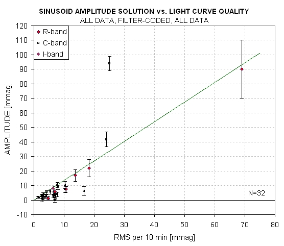
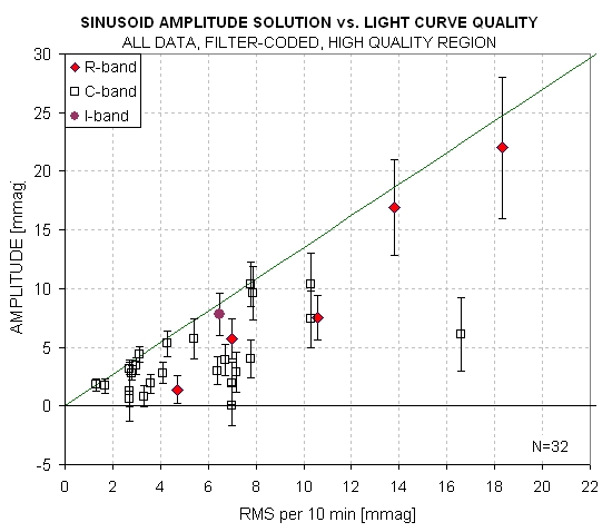
Figure 8a. Sinusoidal amplitude versus LC noisiness
(RMS10) for all 30 targets that have been fitted for a sinusoid variation.
The line is a suggested "upper envelope" having the equation: Amplitude
= 1.35 × RMS10.
Figure 8b. Same data except showing only the high-quality
LCs.
These plots shows a trend suggesting that the poorer the
LC quality the larger the fitted sinusoidal amplitude. Extrapolating
back to a perfect LC (RMS10 = 0) suggests that there would be no
sinusoidal variation. A more accurate description is that an envelope
exists below which are fund all sinusoid amplitudes (with one exception
ou tof 30 cases). This implies that none of the measured amplitudes
are "real" - with the possible exception of one LC WD2134+293, discussed
below). In other words, essentially all plotted amplitudes are "spurious."
Could the envelope slope be the coefficient we're searching
for? The envelope slope is 1.35. Stated another way, spurious sinusoid
amplitude fits can be as high as 1.35 ×RMS10.
The next figure is a target-color-coded plot of all 30 PAWM
sinusoid fit solutions.
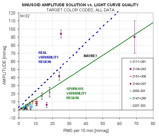
Figure 9a. Sinusoidal amplitude versus LC noisiness
for all 30 cases in the PAWM archive (up until 2010.09.02), with suggested
regions for "spurious" amplitudes, "maybe real" amplitudes and "real"
amplitudes.
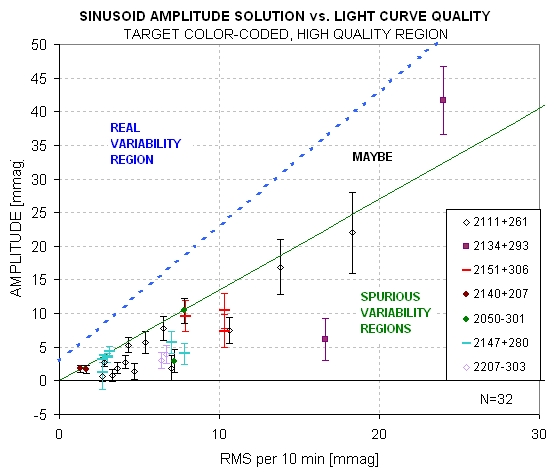
Figure 9b. Same data except showing only the high-quality
LCs.
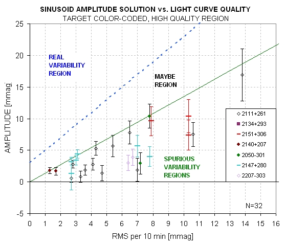
Figure 9c. Same data except showing only the high-quality
LCs.
Let's make a distinction between "high spurious"
and "low spurious" in order to identify LCs that have very small systematic
effects (and low spurious amplitudes) as opposed to those with high systematics
(and high amplitudes). In the next figure the border region between "spurious"
and "maybe" is assigned its own region.
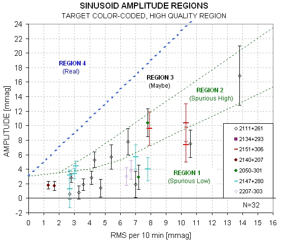
Figure 9d. Four regions ame data except showing only
the high-quality LCs.
These four regions will be used in categorizing LC variability
(starting 2011.09.04). So far, 30 of the 32 stars that have been subjected
to sinusoid fitting are located in "spurious" regions 1 and 2. In
the "What's New" web page, where I give one-liners for each LC that's
been processed, I will include a region number and include RMS10 and amplitude
information in the following way: variability "spurious high" (xy =
2.6/3.4). The xy entry gives the x and y coordinates in the above
figure, which is to say that x = RMS10 and y = amplitude. Thus, in this
example, RMS10 = 2.6 mmag and amplitude = 3.5 mmag.
Fig. 7a shows an LC in the "real" region, WD2134+293 (2011.08.17
by Srdoc), which was the subject of targeted follow-up observations
because of it's apparent non-sinusoidal, 0.18 magnitude variation.
I will adopt the following criterion for tentatively identifying
variability as possibly real (the boundary between Region 3 and 4):
Variation is Possibly
Real if Amplitude > 1.45 × (RMS10 - 0.2 mmag)
As more PAWM targets are observed this criterion equation
will probably be modified.
Prof. Eric Agol Simulation
To check up on what sort of noise might cause the correlations
you are seeing, I created a series of 6 hr. damped random walk light
curves with a range of noise levels. A damped random walks is a random
walk that returns to the mean over some specified timescale
(Zeljko Ivezic likes to call this a 'married drunk'); see http://en.wikipedia.org/wiki/Ornstein–Uhlenbeck_process
also called a continuous time first-order autoregressive process,
or CAR(1).
I set the damping to a time scale of 10 minutes, equivalent
to where you are measuring the RMS, and I set the exposure times equal
to 1 minute. For each light curve I computed the RMS over 10 minute
time bins, and I then fit each light curve with a combination of a sinusoid
and a quadratic with time, optimizing the sinusoid starting within
a period range from 30 min to 6 hr. Each light curve is a completely random
realization with the property that the noise is correlated on timescales
on the order of 10 minutes, but becomes less correlated on longer timescales.
The attached plot is the result of this experiment which
shows a strong linear correlation of the amplitude of the sine curve
with the RMS over 10 minutes, similar to the results you are finding
for observer's light curves. The median best-fit period is 100
minutes, with standard deviation 73 minutes, with a range from 30 to
440 min (this is longer than the 6 hr I stated above since I carry out
an Levenberg-Marquardt optimization for the best fit period found initially
in the range of 0.5-6 hr).
Anyways, this exercise maybe shows the plausibility of
the correlation being caused by random correlated noise in the light
curves. I'm not sure what is special about 10 minutes.
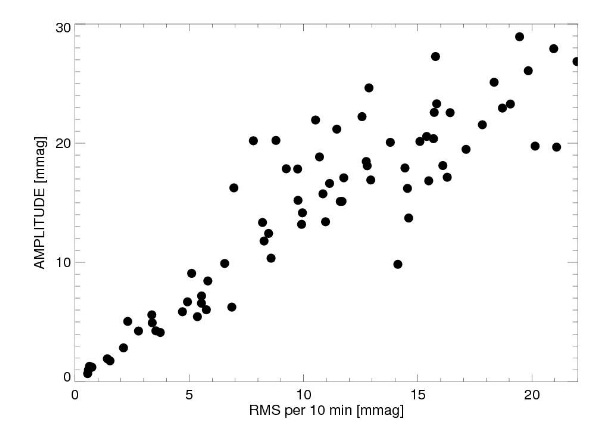
Figure 10. Eric Agol's simulation showing sinusoid
amplitude of fits to a random walk sequence of data.
Bruce Gary Comment
I agree that this simulation could be a good way to represent
actual light curves. There are two aspects of this simulation that
deserve comment: random walk and auto-regression (or "married drunk").
A random walk property can be produced by several real-world
issues. One is the use of an imperfect flat field (no flat field can
be perfect, as described in many places) as the star field moves across
the pixel field during the observing session. Even good autoguiding can't
keep all stars that are in the FOV fixed to the pixel field. Image rotation
due to an imperfect polar alignment (or non-orthogonality of axes) is
one reason. Star locations wander in a way that is uncorrelated with
each other on times scales of seconds when they are a few 'arc apart, so
their average location relative to each other isn't exactly the same for each
exposed image. Image scale can vary slightly as the telescope tube shrinks
from cooling during an observing session. The wavelength passband changes
with air mass differently for stars having different colors. These are a few
ways that systematic effects related to flat fields can insinuate themselves
into a long observing session with timescales of minutes to hours.
Another category that can simulate random walk effects is
produced by varying "atmospheric seeing." As the seeing changes each
star's PSF will vary. When a star is close to the edge of a photometry
aperture sky background annulus it can cause variable fading of the flux
of the star being measured (in the signal aperture circle) because of
the nearby star's PSF spilling into the background annulus. Seeing will
vary on all timescales.
All of these systematic effects become "auto-regressive" in
the final light curve because my fitting procedure uses "temporal
trend" and "air mass curvature" as free parameters. This guarantees
that a fitted LC will minimize the longest timescale components of
any of the random-walk systematic effects. I like the term "random
walk with an elastic leash" becuse it captures the essence of everything
I've just described.
It should be mentioned that the coefficient relating "spurious
sinusoidal amplitude" and "RMS10" should vary with season, and be slightly
different for each observatory. For example, every observatory will
have different atmospheric seeing behaviors, which will vary with season
differently from other observatories. Some telescope tubes don't shrink
as they cool, so image scale changes won't be a problem for them. Etc.
Therefore, I am not surprised that Prof. Eric Agol's simulation
captures the essence of the real-world relationship that I have labeled
"Region 2" in Fig. 7d.
Light Curve Noisiness Comments
A light curve's "noisiness' can be considered to come from
4 sources:
1) Poisson noise
2) Thermal noise
3) Scintillation
4) Systematics
Poisson and thermal noise are straightforward to calculate,
and they can even be calculated as a function of time during a light
curve. Scintillation varies on hourly and daily timescales; however,
changes during an observing session are due mainly to changing air mass.
Scintillation has a typical dependence upon air mass, telescope aperture,
exposure time and site altitude, so an estimate can be made of expected
scintillation versus time during an observing session. Actual scintillation
can differ from estimated (typical) scintillation by a factor of 2 or
3 at any given time. Systematics can't be estimated in any straight-forward
manner. Since total noisiness versus time during an observing session
can be determined it is possible to compare this with the two components
of noisiness that can be determined (Poisson and thermal) to infer the
value of the two components that can't be determined (scintillation and
systematics). Or, since scintillation can be estimated, it is possible
to infer the level of systematics noise by orthogonally subtracting the
orthogonal sum of Poisson, thermal and scintillation from measured total
noise.
RMS10 is measured noise based on that part of the light curve
with air mass < 2 (an arbitrary air mass cut-off choice). It is possible
to calculate RMS versus time during a light curve , and therefore infer
the systematics component of noise as a function of time, but I haven't
done this yet. Whenever I process photometric measurements to produce
a light curve I calculate Poisson and thermal noise, estimate scintillation,
and compare their orthogonal sum with measured noise, RMS10. (All of
these noise levels are entered into an information box of the light curve
plot, as illustrated in the next figure.) The difference between the
expected noise level and measured noise level can be attributed to either
scintillation or systematics. In theory, therefore, there is a way to
estimate the level of systematics for a light curve.
The first three sources of noisiness are "stochastic" and are
expected to have a negligible correlation with spurious variations.
The "systematics" source should dominate this correlation. Consider the
following LC showing a partitioning of LC noise.
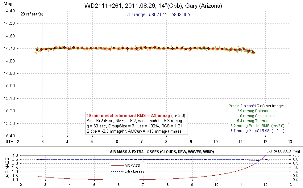
Figure 11. Example of LC showing RMS noise components.
Individual images exhibited an RMS noise of 7.7 mmag, whereas 6.2 mmag
was predicted using calculation of Poisson and thermal noise and a typical
level for scintillation.
In this example the measured RMS for individual images (RMSi)
was slightly larger than the predicted value, which is based on calculated
Poisson and thermal components and an adopted typical scintillation
component. Since in this case RMSi was dominated by the thermal component,
which can be calculated accurately, the total measured noise is insensitive
to the assumed level for scintillation. Therefore, we can use the orthogonal
difference between RMSi measured and RMSi predicted as an estimate of
the level for the systematic noise component. For this example, RMSi
systematic = 4.6 mmag. When a sinusoid fit is permitted for this LC a
spurious sinusoidal amplitude of 1.3 ± 0.6 mmag is found. According
to the explanation that we're developing here to account for spurious
variations there should be a proportionality between the 4.6 mmag "RMSi
systematic" and the 1.3 mmag "spurious sinusoidal amplitude." I suspect
that if a large number of LCs with the noise information calculated could
be analyzed, and if a scatter plot were created relating "spurious sinusoidal
amplitude" to "RMSi systematic," there would be a better correlation than
exists in Fig. 7 ("spurious sinusoidal amplitude" versus RMS10).
A small detail about any future analysis of the type just described
is that a better metric for "spurious variation" should be employed
than "spurious sinusoidal amplitude" because the latter can be expected
to depend on LC length. The longer the LC, the smaller the sinusoidal
amplitude (since systematics are unlikely to have a sinusoidal pattern
with a constant period). A "spurious variability" parameter should be
created for this purpose.
A project for the future is to compare "spurious variability"
with "RMS systematic" for a large number of properly processed LCs.
Proper processing means measuring the noise level on a sampling of images
(in areas without stars) throughout the observing session, for determining
the "thermal" component of the target star's RMSi, and also calculating
the target star's Poisson noise using several reference stars and the correct
equation for predicting the target star's Poisson noise. All of this is
explained in my book, Exoplanet Observing for Amateurs: Second Edition
(link). If there's a positive
correlation between "spurious variability" with "RMS systematic" then
this would provide support for the speculation in the previous section
of this web page, attributing "random walk with an elastic leash" as
the cause for "spurious sinusoidal amplitude." And if such a relation
exists it might provide a way to more accurately predict an expected "spurious
variability," which in turn can be used to more reliably determine the
presence of real variability.
Overlappint
Light Curve Results
It's been difficult to get an overlapping pair of LCs to check
for similar brightness variation structure, and finally we have a
few cases to work with.
Case 1 - YES
The first is a set of LCs that do indeed exhibit real variatios
with a constant period. On Sep 9 WD2359-434 was observed by TG Tan (Perth)
and Paul Tristram/Akihiko Fukui (NZ). The one by Tan had negligible
systematics so that what's hown here:
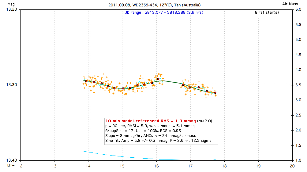
Figure 12. TG Tan's LC, showing a sinusoidal variation with
period 2.6 hours and amplitude 5.8 ± 0.5 mmag.
After several more observations I was able to phase-fold all (good
quality) data to obtain the following LC:
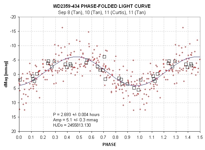
Figure 13. Phase-folded LC for WD2359-434.
Case 2 - NO
Consider the following LC, that anyone can see exhibits a sinusoidal
variation.
Figure 14a. Convincing-looking sinusoidal variation.
Now look at a LC taken at essentially the same time a few hundred miiles
way.
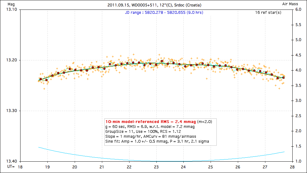
Figure 14b. Convincing-looking non-sinusoidal variation. The
curvature is most likely due to the target star being bluer than the reference
stars.
What can account for these two vastly different LC shapes? I don't
know!
Case 3 - NO
Here's another case of misleading sinusoidal variations in LCs of the
same target on the same date.
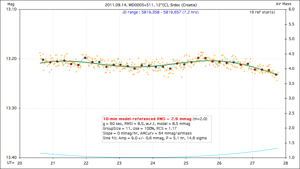
Figure 15a. A nice-looking sinusoidal variation.

Figure 15b. Another nice-looking sinusoidal variation, on same
date, though with smaller amplitude.
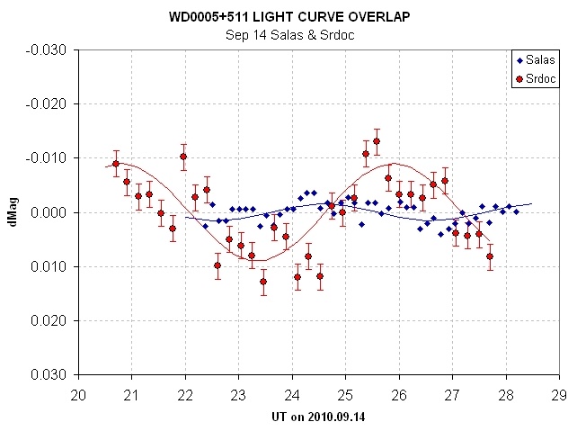
Figure 15c. Overlapping the above two LCs shows a lack of corroboration.
Case 4 - NO
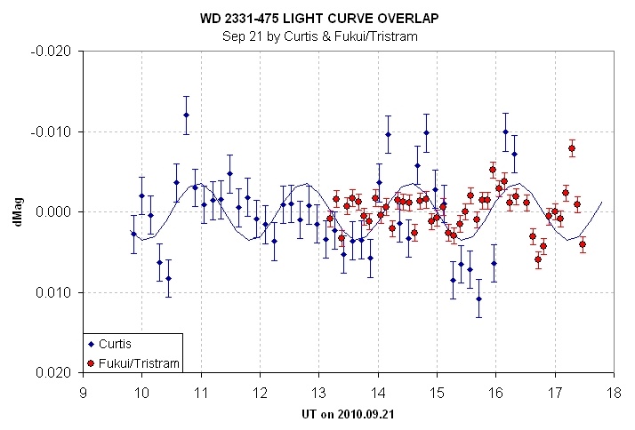
15d. Another example of lack of corroboration of structure.
UCAC3-Based V-Magnitudes
After discovering that one of the V-mag entries in the
Villanova Catalog was in error by ~ 2.0 mag's, which caused one observer
to waste a night observing a target that was too faint for his telescope,
it became necessary to devise an alternate method for deriving a target's
V-band magnitude. The CMC14 catalog of r'-band magnitudes, combined with
2MASS J and K magnitudes, provide very accurate converted magnitudes most
of the time (V-mag SE = 0.020 mag, see http://brucegary.net/dummies/method9.htm).
However, the CMC14 catalog has 3 limitations relevant to PAWM: 1) it is
limited to a declination range of -30 to +50 degrees, so it could not be
used for southern hemisphere targets; 2) converting r'-mag to V-mag produces
outliers ~ 6% of the time, and 3) stars fainter than r'-mag ~ 14.5 are
insufficiently accurate to justify conversion. A safer, though less accurate
procedure, is to perform a conversion using measurements made with a passband
closer to V-band and that is useable for fainter stars. The UCAC3 meets
this need since their passband is intermediate between V- and R-band and
they are useable to ~16.3 mag.
One simple method for obtaining UCAC3 magnitudes is to use the planetarium
program "C2A" ("Computer Aided Astronomy" by Ph. Deverchere, free download
at http://astrosurf.com/c2a/english/index.htm).
An example use of C2A is shown below:
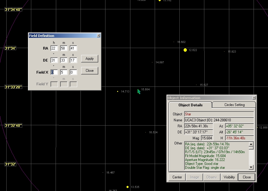
Figure 16. Planetarium program C2A screen capture showing
UCAC3's aperture magnitude for a star at 22:58:41 +31:33:17 (WD2256+313).
The "Aperture Magnitude" is 16.222. The "Fit Model Magnitude" has been
found to be less reliable, so it is ignored. By scrolling down the Object
Information window we note that J = 12.305 and K = 11.460. The SuperCOSMOS
magnitudes for B, R2 and I are also available, but I have shown that they
contribute nothing useful for the task of deriving V-mag. In the next
paragraph I describe how I obtained the conversion equation: V-mag
= 0.69 + 0.925 × UCAC3a + 0.582 × (J-K), where UCAC3a is UCAC3
"Aperture Magnitude." Using this equation yields V-mag = 16.19 ±
0.08 (where the SE is described in the next paragraph also). I've shown
that the outlier rate using this procedure is probably < 1%. For comparison,
the Villanova Catalog lists a V-mag of 13.96 (taken from a publication),
and this is surely too bright by ~ 2 mag based on actual observations (with
a clear filter).
My analysis was inspired by a poster by Joe Garlitz, who used 77 Landolt
stars to derive the following equation: V-mag = 0.796 + 0.917 ×
UCAC3a + 0.636 × (J-K), RMS = 0.079 mag. He, in turn, must have
been inspired by an earlier publication by Hristo Pavlov (2009), who compared
17,000 LONEOS V-mag's to produce the conversion equation: V-mag = 0.83
+ 0.917 × UCAC3a + 0.529 × (J-K), RMS = 0.08 mag. I used
a database of all 92 standard stars with Landolt (2009), SDSS (Smioth et
al, 2002) and UCAC3 magnitudes. I evaluated the use of SuperCOSMOS B, R2
and I magnitudes as additional independent variables, but they contributed
an insignificant improvement to the V-mag accuracy. I also evaluated the
use of higher powers of star color (J-K), but they also had no significant
contribution to converted V-mag accuracy. I also evaluated using UCAC3 "Fit
Model Magnitude" instead of UCAC3 "Aperture Magnitude", but this lead to
a slightly worse RMS for converted V-mag. Here's my final result, plotting
converted V-mag residuals versus star color J-K:
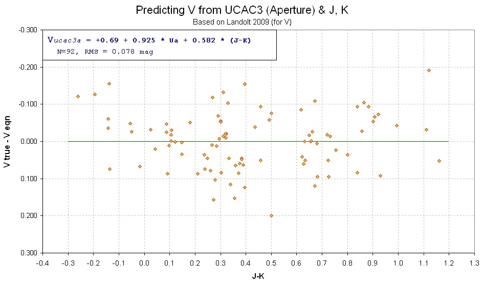
Figure 17. Residuals of my V-mag derivations using UCAC3
"Aperture Magnitude" (referred to as "Ua" in the figure's info box) and
J-K star color, versus star color.
Here's my conversion equation compared with the other two similar equations:
V-mag = 0.83 +
0.917 × UCAC3a + 0.529 × (J-K), RMS = 0.08 mag,
using 17,000 LONEOS V-mag's. Hristo Pavlov (2009)
V-mag = 0.80 + 0.917 × UCAC3a + 0.636 × (J-K), RMS
= 0.079 mag, using 77 Landolt stars. Garlitz (20??)
V-mag = 0.69 + 0.925 × UCAC3a + 0.582 × (J-K), RMS = 0.073
mag, using 92 Landolt stars. Gary (2011)
Debris Disk Animation
Manuel Mendez produced this animation to illustrate one scenario of a debris
disk orbiting in front of a white dwarf star. It should be considered an
"artistic representation" since it is not based on a physical model.


References
Smith, J. Allyn, et al, 2002, AJ, 123, 2121-2144.
Landolt, Arlo U., 2009, AJ, 137, 4186-4269.
WebMaster:
B.
Gary. This site opened: 2011.07.18. Last Update: 2011.09.30