Near Earth Object Rotation Light
Curves and Magnitudes
Observations
by Bruce L. Gary, Hereford, AZ
Summary of RLC Results
NEO # & name Dates w/
Observations
2013 XY8
3C10
Apophis
(2004 MN4) Many dates
5693 93EA
9525, 9528, 9529, 9601, 9603, 9604
138883 00YL29
9501,9505,9506,9508
5011 Ptah
9423, 9422, 9421,
9420, 9419
010416 Kottler
8b20, 8b21, 8c28,
8c29, 8c30, 8c31, 9101, 9102, 9108, 9110, 9111, 9112, 9113
2006SZ217
8c11
1620
Geographos 8b04
2335 James
8b15
162900
8b18, 8b17
Introduction
This web page is meant to record a series of observations of NEOs
with the goal of establishing their rotation light curves (RLC)
and r'-magnitudes. The list of NEO candidates is provided by Brian
Skiff, of the Lowell Observatory.
Links on & from this Web Page
Telescope
calibration (HAO example)
Observing
& image analysis procedures
Sample
RLC Result
Summary of
Results
Hardware, Observing & Image Analysis Procedures
The entire procedure for obtaining RLCs can be thought of as three
parts: observing, image analysis and data analysis.
Hardware. The telescope is fork-mounted on an equatorial
wedge (no meridian flips for me!). In order to reduce image rotation
during an observing session the telescope's polar axis has been
adjusted with an accuracy of ~2 'arc. MaxIm DL (v 4.62, later 5.03)
is used to control the telescope, wireless Craycroft style focuser,
image stabilizer (SBIG AO-7) and CCD camera (SBIG ST-8XE). A
tip-tilt image stabilization mirror (A SBIG AO-7) is used to keep
the star field fixed to the CCD's pixel field.
Master Flat. At least 20 flat field images are made starting
shortly after sunset. Exposure times are adjusted manually to keep
the maximum counts within the range 40,000 to 50,000. Each flat
field exposure is calibrated using a dark frame exposure with the
same exposure time. I stop taking flats when exposure times exceed
~20 seconds. Only those flat field frames with exposure times
greater than 1 second are used in producing a master flat for that
night. I use median combine with level adjustment,
and sometimes and also use the average flat (provided I don't see
artifacts
in any of them). Before starting the flat field exposures I set the
CCD
cooler to about half way between ambient and what I expect to
achieve for
asteroid observations. I also adjust the focus to what I expect
would be
the correct setting for the telescope's temperature (based on
previous
nights of focus versus temperature calibrations). I adhere to the
rule
"Every night must have it's own set of flat fields!"
Master Dark. I'm more relaxed about using a previous night's
master dark frame than a master flat frame. However, I try to use a
master dark that was made using the same CCD temperature setting as
will be
used for the asteroid observations, and I also require that the
exposure times be approximately the same. Calibration of asteroid
images employ aut-scaling to adjust for both.
Master Bias. I use a master bias frame that is within
a few weeks old. It is made from ~20 bias images.
Observing Procedure. Asteroid observations are
started ~55 minutes after sunset. This corresponds approximately to
"nautical twilight." The CCD's FOV is chosen so that a bright star
is
within the autoguider's FOV ("bright" means 12th mag). When mirror
movements
exceed 10% of its range of motion the observing program nudges the
telescope drive motors. Exposure times are typically 100 seconds,
which is short enough to assure that asteroid motion during the
exposure is much smaller than typical PSF FWHM (3.0 to 5.0 "arc for
100-sec exposures). Typically only a few stars are saturated for
this exposure time (my CCD is linear up to ~52,000 ADU).
Image Analysis. More later...
Calibration. Most of these observations are made with a
Celestron 11-inch telescope located inside a "sliding roof
observatory" at my Hereford, AZ site (MPC observatory code G95).
Some were made with a Meade
14-inch, but it's controller card failed 2008 December 2. Each
telescope
is used unfiltered, but the effective bandpass wavelength is
similar
to the r'-band's effective wavelength. But since unfiltered is
much broader
than r' it is important to not use stars for reference that differ
greatly
in color from that for asteroids. For example, it has been
suggested that since asteroid color is typically J-K = 0.42 (V-R =
0.40, g-r
= 0.57) only stars with a similar color should be used for
calibration.
I accept stars with J-K between 0.19 and 0.65 (corresponding to
B-V between
~0.38 and 1.05). The Carlsberg Meridian Catalog is used for
assigning r'
magnitudes to ~ a dozen reference stars. Here's a plot of the
correction
needed to convert apparent r'-mag to true r'mag versus star color
for my
Celestron 11-inch telescope.
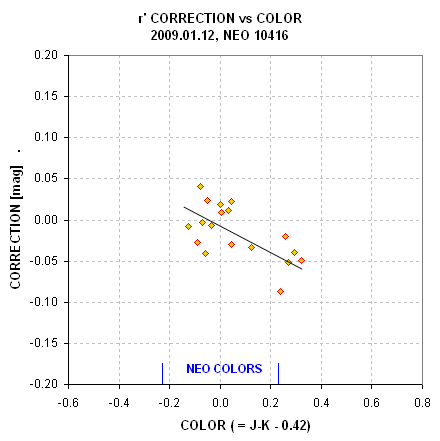
Example of true r'-mag minus apparent r'-mag versus star color.
The range of colors between the blue ticks are used as a
criterion for accepting a star's correction.
Light Curve Creation. Excel...
Folded Rotation Light Curve. B...
Sample Result
- 1620 Geographos
The following RLC is used to illustrate the
results for one NEO. The purpose of this project is to compile a
list of r' magnitudes, periods and variation amplitudes for NEOs
that have not already been observed for this purpose. 1620
Geographos is a well-known, high amplitude RLC NEO, so it serves
here to illustrate what this project endeavors to accomplish in
the context of previous observations. My intent is to conform to
the format given here for all future NEO rotation light curves.
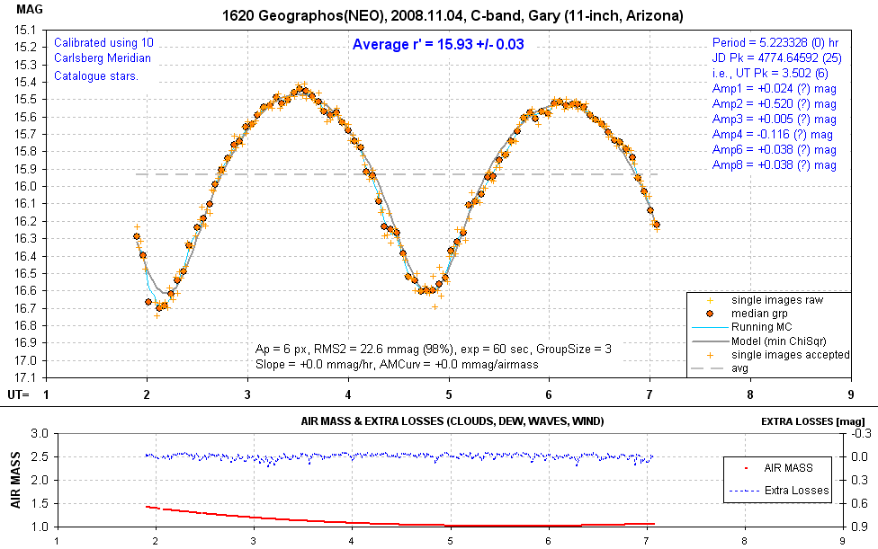
Rotation Light Curve of 1620 Geographos. A detailed
explanation is given in the text. 8b04GBL1 (data
file for download)
The lower panel plots air mass and "extra
losses." The measured flux from a dozen or more nearby stars is
fit by an extinction model and the residual flux is interpreted
as a loss. Contributors to loss could be cirrus clouds, dew or
frost accumulation on the corrector plate, or PSF broadening due
to seeing changes, focus degredation or wind shaking the
telescope. Since
a small and fixed photometry aperture is used to process all
images for an observing session changes in FWHM will produce
changes in "loss." The extinction model is fit to the sum of
fluxes of all nearby stars. In addition to the normal extinction
term, K [magnitudes/airmass], a temporal term is available for
use, as necessary. In this example there were negligible losses
because the sky was clear, humidity was low,
winds were calm and seeing didn't vary much during the observing
session.
The upper panel there are 4 plots. First, a magnitude from each
image employs small orange corsses. Groups of 3 of these are
median combned to produce the large red circle symbols. A
running median combine is shown by a blue trace. Finally, a thin
black trace is a "model fit" that employs the following
parameters: average r' magnitude, rotation period, amplitude of
periodicity having period of 1/2 rotation period (Amp1),
amplitude of periodicity with period 1/4 rotation period (Amp2).
In addition, there are 3 parameters related to calibration and
observing conditions: offset, slope [magnitudes/hour] and air
mass curvature [magnitudes/airmass]. Using the model fit it is
convenient to calculate a "period average magnitude" that is
unaffected by the observing session not exactly equaling a
rotation period (or unequal spacing of observations). The
information box in the lower part of this panel gives the
photometry aperture radius (in pixels, usually ~1.5 to 2.0 x
FWHM), the 2-minute equivalent RMS of the measurements (in
mmag), the percentage of measurements that were used after
rejecting data that exceeded a loss criterion
and neighbor RMS (outlier) criterion, the exposure time for each
image,
the group size used in producing the large red circle symbols
(median
combine), the slope parameter and the air mass curvature
parameter. All graphical presentations of NEO RLCs will have
this format.
Finally, below each graphical RLC there will be a link for
downloading a data file of the measurements. The format will
consist of header lines (object, filter, observer name, etc) and
data columns for JD, magnitude and loss.
WebMaster: B. Gary. Nothing on this web page is copyrighted. This
site opened: 2008.11.16, Last Update: 2014.01.10