Introduction
The HAO is located in Southern Arizona, in the unincorporated community of Hereford (11 miles south of Sierra Vista). The coordinates are Lat = +31.452. EastLon = -110.238, altitude = 1420 meters ASL. Two telescopes are in use at various times, a 14-inch Meade LX200GPS and a 11-inch Celestron CPC1100. The 14-inch is in a sliding roof observatory (SRO),.
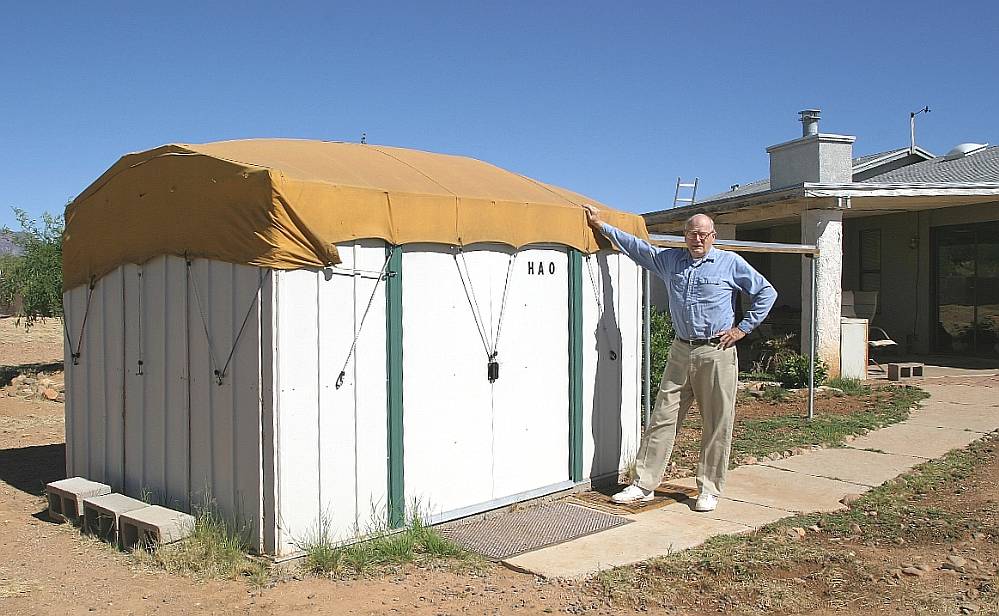
Figure 1. Hereford Arizona Observatory (HAO) with owner Bruce L. Gary.
The SRO shown currently houses the 14-inch telescope (the SRO for the 11-inch has not been built yet). Underground cabling (100 feet) allows for control of the telescope and CCD using a computer in the house. The focuser is wireless, and a survelance camera (audio and video) is also wireless.
Links on this Web Page
Optical Configuration
CCD
Observing Procedure
Image Analysis
Spreadsheet Data Analysis
Telescope Calibration
Optical Configuration
The 14-inch is configured with a Craycroft style wireless focuser (built by Starizona), a Celestron focal reducer, a SBIG AO-7 tip/tilt image stabilizer and a SBIG ST-8XE CCD. The CCD chip is a KAF1602E, with an array of 1530x1020 pixels, each 9 micron square. Next to this main chip is a smaller ST-237 guide chip which is used by the AO-7 for image stabilization. The placement of the focal reducer lens is close to optimum for optical quality and produces an EFL = 1688 mm, corresponding to f/4.75. The image scale is 1.10 "arc/pixel, and the FOV = 28.0 x 18.7 'arc. "Seeing" is typically 3.5 "arc FWHM (2.3 to 4.5 "arc) so the requirement of FWHM > 3 pixels is usually met. The polar axis has been aligned to better than 0.1 degree accuracy. This assures that image rotation during an observing session is small - which in turn minimizes systematic errors due to use of imperfect flat fields..
CCD
The main chip is supposed to have a gain of 2.3 photoeleectrons per ADU, though I measure 2.73 ± 0.03 photoelectrons/ADU. I've measured the read noise to be 18.9 ± 0.2 photoelectrons, or 6.9 ± 0.1 ADU. A TEC cools the chips to ~25 C below ambient. For faint objects (negligible Poisson noise from star photons and negligible scintillation) a typical pixel noise is 7 ADU for a 30-second exposure. This noise level is produced by dark current, sky background and read noise.
Observing Procedure
When a NEO is selected for observation I download orbital elements for it from the MPC site http://www.cfa.harvard.edu/iau/MPEph/MPEph.html and import it to TheSky/Six. This helps plan observations because it is necessary for the NEO's motion during the observing session to be within one FOV setting. Sunset time is checked, the NEO's observing window is determined and an observing schedule is recorded.
I use MaxIm DL 4.62 for controlling the CCD, telescope and focuser. An observing log is kept for recording everything that could possibly be relevant in understanding funny results later.
Shortly after sunset the cooler is set to ~ 10 C below ambient and after the TEC settles a set of ~ 20 flats (unfiltered) are made using a diffuser over the telescope aperture ("double T-shirt" variety). Exposure time is changed as needed to keep maximum counts within the range 40,000 to 50,000, which is below the level where linearity begins to fail. Darks are made with each flat. Flats are later combined (median & average), in groups of <2 seconds exposure and > 2 seconds. The later group is inevitably chosen for use. The average and median versions are compared to verify that there are no cosmic ray artifacts in the average version. If they're both clean then their average is used. The cooler is then set to ~25 C below ambient, after which there's ~30 minutes for a snack dinner.
Star alignment is checked when it's dark enough for visual sighting of the brighter stars i nthe sky. Observations of the NEO are begun at ~ 55 minutes after sunset if the object is above ~ 25 degrees elevation. An exposure time is selected that assures two things: none of the desireable stars are saturated and NEO motion is small compared with FWHM (usually ~ 1 minute). The FOV is positioned so that the autoguider chip has a star with V-mag < ~11; this assures that the AO-7 will be able to update at ~ 1 Hz. Lately the AO-7 has performed well for a stretch of many hours without losing the autoguide star. Nevertheless, since it is not completely reliable I monitor its performance at frequent enough intervals that if has lost track I can manually nudge the telescope motors towithin range of the AO-7 mirror. It's also important to monitor focus at least once per hour during evening cooldown because my tube contracts as it cools. I can tell which focus direction is required from the PSF shape/orientation; I can also consult a plot of best focus setting versus focuser temperature based on previous obserivng sessions. Since I'm old and need my sleep I either quit observing shortly after midnight or go to bed early and set an alarm clock for hourly wakeups to check focus and autoguiding. At the end of the observing session I take about 20 darks using the same exposure time (and cooler setting) that were used for the NEO observations.
Image Analysis
Images are processed using MaxIm DL. A data reduction log is maintained. Images are processed in groups of ~ 150. Dark and flat calibrations are followed by star-alignment using a "master image" (that has been plate solved). The same master image is used for all 150-image groups; this means that when they are saved after star alignment they can be processed again with assurance that all images have the same star alignment. AFter star alignment I add an "artificial star" in a 64x64 pixel upper-left corner of each image. The articifial star has FHWM = 3.789 pixels and a peak ADU of 65,535 counts.
Spot checks of FWHM for images throughout the osberving session are used to select a most-likely aperture photometry radius. Typically FWHM ~ 3.5 pixels, so the most-likely aperture radius is ~6 pixels (i.e., radius ~ 1.6 x FWHM, as Skiff suggests and as I have determined is optimum independently). Photometry is done using aperture radii that span the most-likely radius (eg, 5, 6 and 7 pixels). A photometry gap width is chosen that is about the same as the most-likely radius, and a sky background annulus is chosen to be slightly larger. The radius, gap and annulus values are typically 6, 5 and 8 pixels. Note that the area of the sky background for this choice is ~7 times the area of the signal circle, which means that measurement stochastic noise (due to dark current, sky background level and readout) are dominated by signal aperture readings. The MaxIm DL photometry tool is set to "snap to centroid." It isn't necessary to specify "Use star matching" because all images have already been aligned so that all stars are at the same pixel location in each image. The first and last images are used to specify a "moving object" corresponding to the NEO location for all images. The artificial star is used as "reference." Then a set of ~ 20 unsaturated stars are specified as "check stars." The same set of check stars is used for all groups of 150 images (using an inverted version of the master image with pencil notations). Most of these check stars will later be identified as Carlberg Meridian Catalog stars, and they will eventually serve as reference (in the spreadsheet phase of analysis). When all so-called "check stars" have been selected the photometry measurements made by the MaxIm DL photometry tool are recorded as CSV-files. It is simple to change the signal aperture and repeat the CSV-file recording, and this is done for aperture radii that neighbor the most-likely signal aperure radius.
Spreadsheet Data Analysis
A spreadhseet that has been used for exoplanet LC generation has been modified for use with asteroids. The CSV-files are imported to an import worksheet. Another worksheet is used for calculating air mass from the object's RA/DE, site Lat/Lon and CSV-file JD. A worksheet is devoted to determining an extinction model fit that makes use of the total flux from all "check stars" (extinction per airmass, offset and temporal rate of change). A provision is made for specifying which of the "check stars" are used for reference (using the extinction-corrected star magnitudes). All "check stars" can be displayed in a plot of extinction-corrected magnitude after adjusting for the set of "check stars" used as reference. This permits Delta Scuti stars to be identified ("vermin of the sky" for asteroid people). It also permits identification of "check stars" that misbehave for other reasons (e.g., too near FOV edge and flat field with image rotation caused systematic drift). When a sub-set of "check stars" have been tentatively chosen for use as reference (using their departures from their average for adjustments) criteria are specified for rejecting data due to 1) high unexplained extinction (called "extra losses") and 2) NEO magnitudes that differ from their neighbors by large amounts (called "outliers"). My extinction rejection criterion is usually 0.1 magnitude, and my outlier criterion is adjusted so that about 98% of the remaining data is accepted. This last rejection will inevitably reject the 3-sigma data points, but this is a small penalty for rejecting data affected by the more common defects (cosmic rays, etc).
In order to perform a zero-shift adjustment that puts the NEO magnitudes on a good r' magnitude scale it is necessary to consult the Carlberg Meridian Catalog (CMC14). (Thanks, Brian, for explaining about DS9 and the Carlsberg stars!) The "master image" is imported to DS9 and the Analyze/Catalog menus is opened for selecting the CMC slist. This list is filtered for r'-magnitudes <14.5 and sorted for increasing r'-magnitude (r' > 14.5 do indeed apear to be noisy). The "master iamge" has all CMC stars circled. As entries are highlighted in the CMC list the corresponding circle blinks for awhile (& the image is shifted so the corresponding star is in the center of the image display panel). I note the r', J and K magnitudes in the reduction log whenever one of the CMC stars corresponds to one of the 20 or so "check stars" that were measured by MaxIm DL's photometry tool. After all correspondences of CMC star with "check star" have been recorded, I enter the r', J and K values in the spreadhseet next to each star's measured median magnitude (i.e., where "measured" means corrected for extinction, adjusted for departures of the candidate reference stars {"check stars"}from their average value, and all such candidate reference stars sero-shifted to produce approximate agreement with the object's expected r'-magnitude). I identify "candidate reference stars" (which I've also referred to as "check stars") with J-K colors within the range 0.20 to 0.65 as being close enough in color to the typical asteroid for it to be used in calibrating the present NEO data. For each of these "candidate reference stars" with CMC r'-magnitudes and acceptable colors I note the difference between r'-mag and measured mag. So far there has been amazingly small scatter in these differences (numbering ~ 15). The median od these differences is used to make a final zero-shift adjustment; thjis then places the NRO magnitudes on a calibrated r'-magnitude scale.
Telescope Calibration
I have gotten in the habit of calibrating my telescopes so that a total flux from a star can be instantly converted to a magnitude using a simple equation, such as:
 Eqn 1
Eqn 1
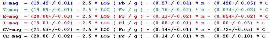
For example, if a 60 second observation of a star that has a flux of 100,000 counts (using a large photometry aperture) using a B-filter at airmass = 1.2, and if I assume the star has a typical color, then the first of the above equations states that B-mag = 11.04. I like having a quick way to convert a star image to an approximate magnitude using a hand calculator. When I have a set of equations like this one I consider the telescope to be "photomeetrically calibrated." The calibration for BVRI requires observations of Landolt star fields. Recently (2008.11.15) I observed the Landolt star field at RA = 21:42 with the 14-inch Meade, unfiltered (my CFW is broken) and repeated the telescope photometry calibration, yielding the following:
 Eqn 2
Eqn 2
I note that the two CR equations differ by 0.28 magnitude. The likely explanation for this is that the first set of magnitude equations were made with a color filter wheel, which extended the backend optics enough to block an outer rim of the 14-inch aperture to an effective 12.3-inches! (Tom Kaye recently pointed out that I might have this problem after he looked into the front of the aperture from near the edge and saw blocking. "Live and learn!")
A similar procedure was done using Carlberg r'-magnitudes:
 Eqn 3
Eqn 3
The "Clear to R-band" zero-shift parameter differs from the "Clear to r'-band" zero-shift parameter by 0.23 magnitudes, which is close to the difference in these two magnitude scales.
In arriving at the color coefficient (the last term in the equation) it was necessary to construct a plot of "discrepancy versus star color" (it's more complicated than this, but let's not get bogged down by details). Here's an example of a typical "discrepancy versus color plot for the 14-inch (when it had a CFW installed):
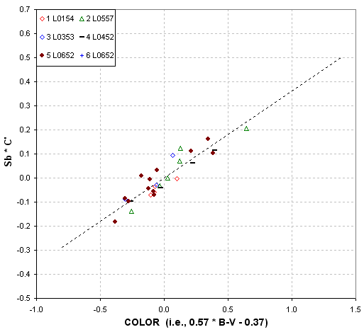
Figure 2. Discrepancy versus star color for B-band measurements of Landolt stars (2008.01.18)
In this plot the so-called discrepancies correlate with star color (defined in a special way, shown in the figure). The residuals from the dashed fit line have an RMS = 0.038 magnitude. For the other bands (V,Rc,Ic) the RMS residuals are typically smaller (because extinction is smaller and SNR is larger).
For the current 14-inch configuration the R-band "discrepancy versus color" plot is shown here:
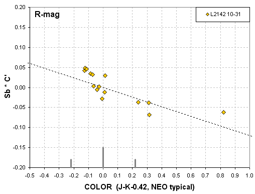
Figure 3. Discrepancy versus star color for R-band measurements of Landolt stars (2008.11.15)
The way color is defined, such that a typical asteroid has color of zero, my color acceptance criterion (stated above) is indicated by the vertical gray ticks at -0.22 and +0.22. Over this range R-band magnitudes will exhibit systematic errors that range from -0.023 to +0.025 magnitude.
For r'-magnitudes, using the Carlsberg data, the following was determined:
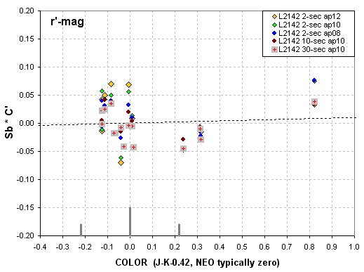
Figure 4. Discrepancy versus star color for r'-band measurements of Carlsberg stars (2008.11.15)
Over the range of my J-K color acceptance criterion r'-band magnitudes will exhibit systematic errors that range from -0.001 to +0.001 magnitude!
The data in this plot is "noisy" and should be repeated using another set of Carlsberg stars.
Conclusion
Procedures have been developed for observing NEOs, processing the images and analyzing the flux readings. A procedure for calibrating the NEO measurements to r'-magnitude has been demonstrated. A crucial part of that calibration procedure is the use of Carlsberg Meridian Catalog stars usin the DS9 program (as suggested by Brian Skiff).
The 14-inch Meade telescope system, configured without a CFW, has been tentatively calibrated photometrically. It is possible to quickly convert a star flux to R or r' magnitude and an assumed (or determined) extinction for the night in question. Almost all Carlsberg stars, regardless of clor, can be used for calibration since the telescope system appears to be essentially color insensitive for converting unfiltered measurements to r'-magnitude.
The HAO is located in Southern Arizona, in the unincorporated community of Hereford (11 miles south of Sierra Vista). The coordinates are Lat = +31.452. EastLon = -110.238, altitude = 1420 meters ASL. Two telescopes are in use at various times, a 14-inch Meade LX200GPS and a 11-inch Celestron CPC1100. The 14-inch is in a sliding roof observatory (SRO),.
Figure 1. Hereford Arizona Observatory (HAO) with owner Bruce L. Gary.
The SRO shown currently houses the 14-inch telescope (the SRO for the 11-inch has not been built yet). Underground cabling (100 feet) allows for control of the telescope and CCD using a computer in the house. The focuser is wireless, and a survelance camera (audio and video) is also wireless.
Links on this Web Page
Optical Configuration
CCD
Observing Procedure
Image Analysis
Spreadsheet Data Analysis
Telescope Calibration
Optical Configuration
The 14-inch is configured with a Craycroft style wireless focuser (built by Starizona), a Celestron focal reducer, a SBIG AO-7 tip/tilt image stabilizer and a SBIG ST-8XE CCD. The CCD chip is a KAF1602E, with an array of 1530x1020 pixels, each 9 micron square. Next to this main chip is a smaller ST-237 guide chip which is used by the AO-7 for image stabilization. The placement of the focal reducer lens is close to optimum for optical quality and produces an EFL = 1688 mm, corresponding to f/4.75. The image scale is 1.10 "arc/pixel, and the FOV = 28.0 x 18.7 'arc. "Seeing" is typically 3.5 "arc FWHM (2.3 to 4.5 "arc) so the requirement of FWHM > 3 pixels is usually met. The polar axis has been aligned to better than 0.1 degree accuracy. This assures that image rotation during an observing session is small - which in turn minimizes systematic errors due to use of imperfect flat fields..
CCD
The main chip is supposed to have a gain of 2.3 photoeleectrons per ADU, though I measure 2.73 ± 0.03 photoelectrons/ADU. I've measured the read noise to be 18.9 ± 0.2 photoelectrons, or 6.9 ± 0.1 ADU. A TEC cools the chips to ~25 C below ambient. For faint objects (negligible Poisson noise from star photons and negligible scintillation) a typical pixel noise is 7 ADU for a 30-second exposure. This noise level is produced by dark current, sky background and read noise.
Observing Procedure
When a NEO is selected for observation I download orbital elements for it from the MPC site http://www.cfa.harvard.edu/iau/MPEph/MPEph.html and import it to TheSky/Six. This helps plan observations because it is necessary for the NEO's motion during the observing session to be within one FOV setting. Sunset time is checked, the NEO's observing window is determined and an observing schedule is recorded.
I use MaxIm DL 4.62 for controlling the CCD, telescope and focuser. An observing log is kept for recording everything that could possibly be relevant in understanding funny results later.
Shortly after sunset the cooler is set to ~ 10 C below ambient and after the TEC settles a set of ~ 20 flats (unfiltered) are made using a diffuser over the telescope aperture ("double T-shirt" variety). Exposure time is changed as needed to keep maximum counts within the range 40,000 to 50,000, which is below the level where linearity begins to fail. Darks are made with each flat. Flats are later combined (median & average), in groups of <2 seconds exposure and > 2 seconds. The later group is inevitably chosen for use. The average and median versions are compared to verify that there are no cosmic ray artifacts in the average version. If they're both clean then their average is used. The cooler is then set to ~25 C below ambient, after which there's ~30 minutes for a snack dinner.
Star alignment is checked when it's dark enough for visual sighting of the brighter stars i nthe sky. Observations of the NEO are begun at ~ 55 minutes after sunset if the object is above ~ 25 degrees elevation. An exposure time is selected that assures two things: none of the desireable stars are saturated and NEO motion is small compared with FWHM (usually ~ 1 minute). The FOV is positioned so that the autoguider chip has a star with V-mag < ~11; this assures that the AO-7 will be able to update at ~ 1 Hz. Lately the AO-7 has performed well for a stretch of many hours without losing the autoguide star. Nevertheless, since it is not completely reliable I monitor its performance at frequent enough intervals that if has lost track I can manually nudge the telescope motors towithin range of the AO-7 mirror. It's also important to monitor focus at least once per hour during evening cooldown because my tube contracts as it cools. I can tell which focus direction is required from the PSF shape/orientation; I can also consult a plot of best focus setting versus focuser temperature based on previous obserivng sessions. Since I'm old and need my sleep I either quit observing shortly after midnight or go to bed early and set an alarm clock for hourly wakeups to check focus and autoguiding. At the end of the observing session I take about 20 darks using the same exposure time (and cooler setting) that were used for the NEO observations.
Image Analysis
Images are processed using MaxIm DL. A data reduction log is maintained. Images are processed in groups of ~ 150. Dark and flat calibrations are followed by star-alignment using a "master image" (that has been plate solved). The same master image is used for all 150-image groups; this means that when they are saved after star alignment they can be processed again with assurance that all images have the same star alignment. AFter star alignment I add an "artificial star" in a 64x64 pixel upper-left corner of each image. The articifial star has FHWM = 3.789 pixels and a peak ADU of 65,535 counts.
Spot checks of FWHM for images throughout the osberving session are used to select a most-likely aperture photometry radius. Typically FWHM ~ 3.5 pixels, so the most-likely aperture radius is ~6 pixels (i.e., radius ~ 1.6 x FWHM, as Skiff suggests and as I have determined is optimum independently). Photometry is done using aperture radii that span the most-likely radius (eg, 5, 6 and 7 pixels). A photometry gap width is chosen that is about the same as the most-likely radius, and a sky background annulus is chosen to be slightly larger. The radius, gap and annulus values are typically 6, 5 and 8 pixels. Note that the area of the sky background for this choice is ~7 times the area of the signal circle, which means that measurement stochastic noise (due to dark current, sky background level and readout) are dominated by signal aperture readings. The MaxIm DL photometry tool is set to "snap to centroid." It isn't necessary to specify "Use star matching" because all images have already been aligned so that all stars are at the same pixel location in each image. The first and last images are used to specify a "moving object" corresponding to the NEO location for all images. The artificial star is used as "reference." Then a set of ~ 20 unsaturated stars are specified as "check stars." The same set of check stars is used for all groups of 150 images (using an inverted version of the master image with pencil notations). Most of these check stars will later be identified as Carlberg Meridian Catalog stars, and they will eventually serve as reference (in the spreadsheet phase of analysis). When all so-called "check stars" have been selected the photometry measurements made by the MaxIm DL photometry tool are recorded as CSV-files. It is simple to change the signal aperture and repeat the CSV-file recording, and this is done for aperture radii that neighbor the most-likely signal aperure radius.
Spreadsheet Data Analysis
A spreadhseet that has been used for exoplanet LC generation has been modified for use with asteroids. The CSV-files are imported to an import worksheet. Another worksheet is used for calculating air mass from the object's RA/DE, site Lat/Lon and CSV-file JD. A worksheet is devoted to determining an extinction model fit that makes use of the total flux from all "check stars" (extinction per airmass, offset and temporal rate of change). A provision is made for specifying which of the "check stars" are used for reference (using the extinction-corrected star magnitudes). All "check stars" can be displayed in a plot of extinction-corrected magnitude after adjusting for the set of "check stars" used as reference. This permits Delta Scuti stars to be identified ("vermin of the sky" for asteroid people). It also permits identification of "check stars" that misbehave for other reasons (e.g., too near FOV edge and flat field with image rotation caused systematic drift). When a sub-set of "check stars" have been tentatively chosen for use as reference (using their departures from their average for adjustments) criteria are specified for rejecting data due to 1) high unexplained extinction (called "extra losses") and 2) NEO magnitudes that differ from their neighbors by large amounts (called "outliers"). My extinction rejection criterion is usually 0.1 magnitude, and my outlier criterion is adjusted so that about 98% of the remaining data is accepted. This last rejection will inevitably reject the 3-sigma data points, but this is a small penalty for rejecting data affected by the more common defects (cosmic rays, etc).
In order to perform a zero-shift adjustment that puts the NEO magnitudes on a good r' magnitude scale it is necessary to consult the Carlberg Meridian Catalog (CMC14). (Thanks, Brian, for explaining about DS9 and the Carlsberg stars!) The "master image" is imported to DS9 and the Analyze/Catalog menus is opened for selecting the CMC slist. This list is filtered for r'-magnitudes <14.5 and sorted for increasing r'-magnitude (r' > 14.5 do indeed apear to be noisy). The "master iamge" has all CMC stars circled. As entries are highlighted in the CMC list the corresponding circle blinks for awhile (& the image is shifted so the corresponding star is in the center of the image display panel). I note the r', J and K magnitudes in the reduction log whenever one of the CMC stars corresponds to one of the 20 or so "check stars" that were measured by MaxIm DL's photometry tool. After all correspondences of CMC star with "check star" have been recorded, I enter the r', J and K values in the spreadhseet next to each star's measured median magnitude (i.e., where "measured" means corrected for extinction, adjusted for departures of the candidate reference stars {"check stars"}from their average value, and all such candidate reference stars sero-shifted to produce approximate agreement with the object's expected r'-magnitude). I identify "candidate reference stars" (which I've also referred to as "check stars") with J-K colors within the range 0.20 to 0.65 as being close enough in color to the typical asteroid for it to be used in calibrating the present NEO data. For each of these "candidate reference stars" with CMC r'-magnitudes and acceptable colors I note the difference between r'-mag and measured mag. So far there has been amazingly small scatter in these differences (numbering ~ 15). The median od these differences is used to make a final zero-shift adjustment; thjis then places the NRO magnitudes on a calibrated r'-magnitude scale.
Telescope Calibration
I have gotten in the habit of calibrating my telescopes so that a total flux from a star can be instantly converted to a magnitude using a simple equation, such as:
Eqn 1For example, if a 60 second observation of a star that has a flux of 100,000 counts (using a large photometry aperture) using a B-filter at airmass = 1.2, and if I assume the star has a typical color, then the first of the above equations states that B-mag = 11.04. I like having a quick way to convert a star image to an approximate magnitude using a hand calculator. When I have a set of equations like this one I consider the telescope to be "photomeetrically calibrated." The calibration for BVRI requires observations of Landolt star fields. Recently (2008.11.15) I observed the Landolt star field at RA = 21:42 with the 14-inch Meade, unfiltered (my CFW is broken) and repeated the telescope photometry calibration, yielding the following:
I note that the two CR equations differ by 0.28 magnitude. The likely explanation for this is that the first set of magnitude equations were made with a color filter wheel, which extended the backend optics enough to block an outer rim of the 14-inch aperture to an effective 12.3-inches! (Tom Kaye recently pointed out that I might have this problem after he looked into the front of the aperture from near the edge and saw blocking. "Live and learn!")
A similar procedure was done using Carlberg r'-magnitudes:
The "Clear to R-band" zero-shift parameter differs from the "Clear to r'-band" zero-shift parameter by 0.23 magnitudes, which is close to the difference in these two magnitude scales.
In arriving at the color coefficient (the last term in the equation) it was necessary to construct a plot of "discrepancy versus star color" (it's more complicated than this, but let's not get bogged down by details). Here's an example of a typical "discrepancy versus color plot for the 14-inch (when it had a CFW installed):
Figure 2. Discrepancy versus star color for B-band measurements of Landolt stars (2008.01.18)
In this plot the so-called discrepancies correlate with star color (defined in a special way, shown in the figure). The residuals from the dashed fit line have an RMS = 0.038 magnitude. For the other bands (V,Rc,Ic) the RMS residuals are typically smaller (because extinction is smaller and SNR is larger).
For the current 14-inch configuration the R-band "discrepancy versus color" plot is shown here:
Figure 3. Discrepancy versus star color for R-band measurements of Landolt stars (2008.11.15)
The way color is defined, such that a typical asteroid has color of zero, my color acceptance criterion (stated above) is indicated by the vertical gray ticks at -0.22 and +0.22. Over this range R-band magnitudes will exhibit systematic errors that range from -0.023 to +0.025 magnitude.
For r'-magnitudes, using the Carlsberg data, the following was determined:
Figure 4. Discrepancy versus star color for r'-band measurements of Carlsberg stars (2008.11.15)
Over the range of my J-K color acceptance criterion r'-band magnitudes will exhibit systematic errors that range from -0.001 to +0.001 magnitude!
The data in this plot is "noisy" and should be repeated using another set of Carlsberg stars.
Conclusion
Procedures have been developed for observing NEOs, processing the images and analyzing the flux readings. A procedure for calibrating the NEO measurements to r'-magnitude has been demonstrated. A crucial part of that calibration procedure is the use of Carlsberg Meridian Catalog stars usin the DS9 program (as suggested by Brian Skiff).
The 14-inch Meade telescope system, configured without a CFW, has been tentatively calibrated photometrically. It is possible to quickly convert a star flux to R or r' magnitude and an assumed (or determined) extinction for the night in question. Almost all Carlsberg stars, regardless of clor, can be used for calibration since the telescope system appears to be essentially color insensitive for converting unfiltered measurements to r'-magnitude.
WebMaster: B. Gary. Nothing on this web page is copyrighted. This site opened: 2008.11.16, Last Update: 2008.11.16