CALIBRATION OF VESTA & CERES OBSERVATIONS AT
HEREFORD ARIZONA OBSERVATORY IN 2014
Webmaster: Bruce L. Gary, Hereford, AZ; USA; Last Update: 2015
Feb 22
This web page describes
the calibration of observations of Vesta and Ceres at the
Hereford Arizona Observatory (HAO) during their 2014
opposition. Dawn spacecraft Framing Camera (FC) filters
were used, so no stars were available that had been
calibrated for these bands. Therefore, Phase 1 for this
project entailed calibrating stars near the Vesta and
Ceres locations using Vega as a primary standard. This, in
essence, amounted to the creation of a new 7-band
magnitude system. For each FC filter the flux of Vega was
transferred to several stars using all-sky calibration
techniques. Phase 2 consisted of observations of Vesta and
Ceres, and these also required the use of all-sky
techniques since none of the secondary calibration stars
were within the field-of-view of Vesta or Ceres images. I
estimate that for all FC bands an accuracy of ~ 3.3 % was
achieved.
Links
Phase 1, Transferring Vega Fluxes to
Secondary Stars
Phase 2, Using
Secondary Standard Stars to Calibrate Vesta and Ceres
Observations
Supporting
Material for Creating a New
Magnitude System (another web
page)
Introduction
The goal of this observational project is to measure
the geometric albedo of Vesta and Ceres. This requires a method
for measuring the flux reflected by the asteroid and comparing it
with what it intercepts from the sun. The flux within a specified
range of wavelengths is related to magnitude by a simple equation,
such that knowing one means you also know the other (see SED for a fuller
description). The approach to measuring an asteroid's albedo
involves comparing its flux at a specific wavelength interval with
the flux from a star whose flux within that same wavelength range
is known. That is equivalent to stating that an asteroid's albedo
involves measuring its magnitude by calibrating it with a star
whose magnitude is known.
Calibrations with a CCD camera are usually performed using
background stars that have calibrated magnitudes listed in a
catalog, such as the UCAC4 catalog that includes APASS BVg'r'i'
magnitudes. If a V-band filter is used, then stars in the same
image as the asteroid that have APASS V-magnitudes are used for
calibration. Since there are always small differences between the
telescope system spectral response function (above the atmosphere)
and the response function used to define a magnitude system, "CCD
transformation equations" are used by the conscientious observer
to provide more accurate calibration of the asteroid magnitude.
When spreadsheets came into common use a simpler alternative to
CCD transformation equations became an option. This involves
constructing a plot of "instrument magnitude minus APASS
calibrated magnitude versus star color of the calibrated star
(such as B-V, or g'-i')." With such a plot, fitted by a magnitude
offset and slope, it is possible to convert the instrumental
magnitude of any target of interest to a calibrated magnitude -
provided the target of interest has a known color (B-V, etc).
Since most asteroids do not have a known color it is commonly
assumed that they are slightly redder than the sun (B-V = 0.64),
which is OK for assigning a provisional magnitude to the asteroid
until its color can be measured. Measuring the color of an
asteroid involves an iterative procedure, which is straightforward
and has fast convergence. Few observers go to the trouble of
making the necessary observations for achieving accurate asteroid
magnitudes, regardless of which band they use. Phase function
plots can be subject to systematic errors produced by this
neglect, and this should be "kept in mind" by anyone using phase
effect data for scientific analysis for deriving regolith
properties.
When using filters that have no analogue in a catalog of
calibrated star magnitudes, such as the Dawn FC filters, these
issues are especially important. Usually it is possible to
construct a phase effect plot without careful attention to CCD
transformations (or their equivalent), since most asteroids have
the same color for all observing sessions used to establish the
phase effect relation. However, such data can be expected to
produce an unreliable zero phase magnitude (H) since all data will
share an unknown calibration offset error. The situation can be
even worse for an asteroid that exhibits changes in color as it
rotates, such as Vesta; unless careful calibration is performed
such an observed phase effect will exhibit subtle systematic
errors affecting phase effect shape as well as the H value.
For these reasons there is merit in creating a magnitude system
designed for use with only the the FC filters for characterizing
the phase effect relations for Vesta and Ceres.
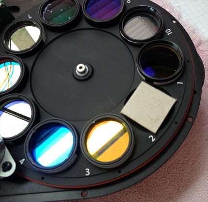
Figure 1. The FC filters in a 10-slot color
filter wheel.
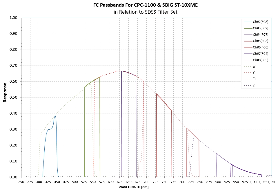
Figure 2. FC passbands compared with SDSS passbands
(g'r'i'z'), multiplied by a typical CCD QE function and
atmospheric transmission function, showing the difficulty in
finding an equivalence between FC filters and SDSS
filter for calibration purposes.(The situation is even worse
comparing FC filters with the Johnson-Cousins BVRcIc
filters).
Phase 1: Transferring Vega Fluxes to
Secondary Standard Stars
This may be hard to believe,
but the following Phase 1 material is the "short version"
describing how I created a new magnitude system for the FC
filters. If anything on this web page isn't explained in
sufficient detail then consider viewing the web page linked to
above under "Supporting Material...", where I treat some basic
concepts for anyone creating a magnitude system.
A new magnitude system was created for each of the 7 FC filters
using Vega as a primary standard for establishing zero magnitudes
(above the atmosphere). Secondary standard stars were calibrated
using Vega; two A0V stars (same as Vega) and several sun-like
stars were included as secondary standards. These secondary stars
were located close to the position of Vesta and Ceres for the 2014
opposition (March through June, 2014). Once calibrated, any of the
secondary standard stars could be used to calibrate observations
Vesta and Ceres since they were all at the same air mass and
observable at the same time. This web page describes how the task
of "deriving a magnitude system" was accomplished and how the same
all-sky calibration techniques were used for calibrating the Vesta
and Ceres observations.
Phase 1 measurements were made
March 16 to 25, 2014 using a Celestron 11-inch (CPC1100)
Schmidt-Cassegrain telescope, with a 10-position CFW and SBIG
ST-10XME CCD. The telescope was inside a dome in my backyard,
and all equipment was controlled from inside my house using
MaxIm DL (v5.3) through 100-foot buried cables to the dome
observatory. Phase 2 observations were conducted with the same
Celestron 11-inch telescope system (March 20 to May 01) and with
a Meade 14-inch Schmidt-Cassegrain
telescope (May 5 to June
20) located in a different dome but using the same
filter wheel and CCD. Additional description of these two
observatories can be found at http://www.brucegary.net/HAO/.
Vega is probably the most-studied
star in terms of flux spectrum, Fλ
[Watts/m2/micron].
The low-resolution spectrum used for this analysis is shown in
Figure 3, and is based on the tabulation by Kurucz (2003).
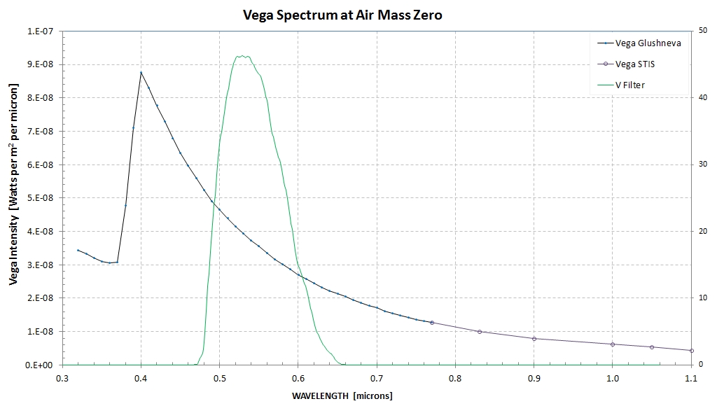
Figure 3. Vega flux spectrum, a primary
standard used to establish flux spectra for a set of secondary
standard stars near the Vesta and Ceres sky location.
The V-band filter bandpass is shown.
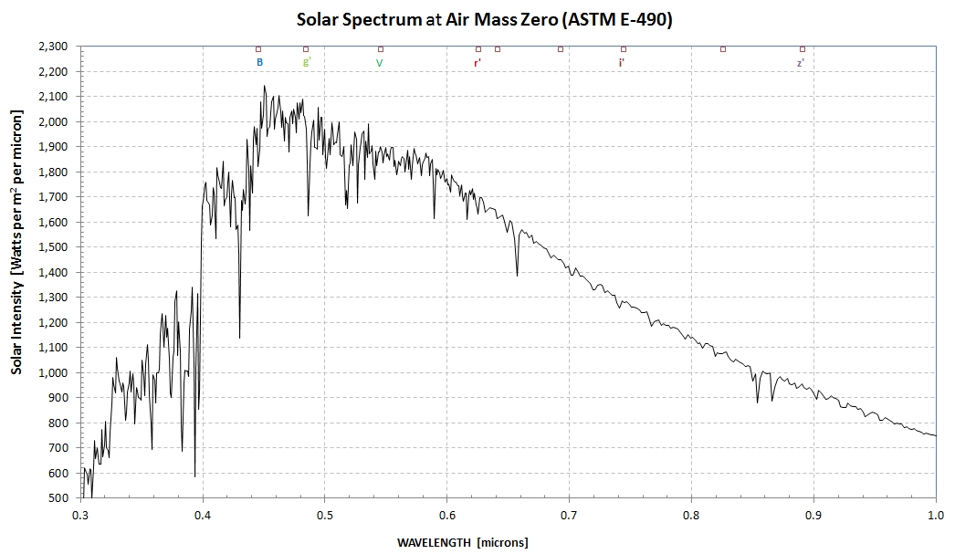
Figure 4. Solar flux spectrum, based on the ASTM
E-490 model. The V filter response function is also shown.
The solar
spectrum, shown as Fig. 4, is also well-established. I use the
"2000 ASTM Standard Extraterrestrial Spectrum Reference
E-490-00" for this analysis. Here's a link to a tabulation of
the Vega flux and solar flux that I use, plus typical
atmospheric transmission, with a 1 nm resolution: link. The Vega and solar
flux spectra are probably more accurate than 1% within the
wavelength region spanned by the FC filters (0.4 to 1.02
micron).
The concept of transferring flux information from a primary
standard star to another one, to be used as a secondary
standard, is straightforward to understand but difficult to
implement. Let's begin with the simple case of the two stars
being next to each other, within a CCD image FOV. The transfer
could be accomplished by measuring the total ADU counts within
a large photometry aperture for each star and taking their
ratio. Some subtleties exist even for this simple case: a good
quality flat field would be required, many such images would
have to be made in order to reduce scintillation and Poisson
noise, and a large number of images would be needed that
sample a range elevation angles in order to remove the effect
of atmospheric extinction producing ratios that vary with air
mass due to the two stars' different spectral slope across the
filter passband. This last effect is important because star
magnitudes are defined in terms of what would be observed from
above the atmosphere.
Imagine, now, the additional observing requirements when the
two stars are in quite different parts of the sky. For
example, when I performed the calibration transfer from Vega
to a set of secondary standard stars near Vesta and Ceres,
during March, Vega would rise through 25 degrees elevation at
1:30 am when Vesta and Ceres were at ~ 60 degrees elevation.
Overcoming this problem is what "all-sky photometry" is all
about. The usual all-sky solution is to observe when both
stars are at about the same elevation at the same time, and go
back and forth observing them in alternation. (For Vega and
the Vesta/Ceres part of the sky, this occurred a couple hours
before sunrise.)
One has to assume that atmospheric extinction is the same in
both parts of the sky, such that extinction at a given air
mass is the same. Since this may be true for some wavelength
regions it is not necessarily true for other wavelength
regions. This is due to atmospheric extinction consisting of
four different sources: Rayleigh scattering, aerosols,
stratospheric ozone and tropospheric water vapor. Rayleigh
scattering is proportional to surface air pressure, aerosol
scattering (and absorption) vary with the burden of dust in
the lower troposphere, ozone absorption varies with the
circulation of stratospheric ozone from the tropics to
mid-latitudes and water vapor varies with the synoptic and
mesoscale circulation of lower tropospheric air masses. The
greatest horizontal gradients of atmospheric extinction are
due to water vapor and aerosols. The best way to overcome
horizontal gradient problems is to repeat observing sessions
on several dates, when presumably the horizontal gradients
will "average out." I observed Vega and the secondary standard
stars on three dates, and achieved similar results -
indicating that horizontal gradients were not a significant
problem during these observing sessions.
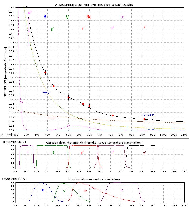
Figure 5. Atmospheric extinction at my observing
site (4670 feet ASL) on one winter date, showing the four
components contributing to extinction.
Another problem associated with transferring calibration from
a bright star to fainter ones is that all exposures must
assure that the bright star is not "saturated" (i.e., with
maximum ADU counts < ~ 50,000) and that the fainter stars
have sufficient SNR to be measured with good precision. Vega
was ~ 100 times brighter than the secondary stars, and I
couldn't expose for a short enough time to prevent saturation
(for even a good CCD camera exposures should exceed ~ 1 second
to maintain accuracy). My solution to this was to use an
aperture mask with a 1-inch hole for Vega observations, and
observe the secondary standard stars without the mask; this
allowed similar exposure times to be used for both. The 1-inch
hole had to be calibrated, and this was done using one of the
secondary stars. By alternating observations of a star with
and without the aperture mask, on two dates, it was determined
that the ratio of "collecting area," unmasked to masked, was
98.63 ± 1.28, or 4.985 ± 0.014
magnitudes. This component of
uncertainty is less important than the transfer of fluxes
from Vega to the secondary standards. Below is a
list of stars considered for use as secondary standards.
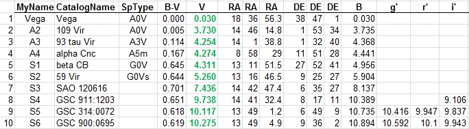
Figure 6. List of stars considered for use during
the calibration transfer phase of observing. A stars and S
stars refer to spectral type A and solar spectral type.
Star #6, in the above list, became the most relied upon
secondary standard star. It is also called 59 Vir (in Virgo).
It has a B-V essentially the same as the sun. This was an
important consideration in placing greater reliance upon it
for the asteroid observations. To the extent that Ceres, for
example, has the same spectrum as the sun there should be
minimal variation in the ratio of Ceres to 59 Vir as
atmospheric extinction changes (due to air mass changes, or
any other atmospheric changes). Another advantage in choosing
59 Vir for the most used secondary standard star is that it
allowed me to switch telescopes, from the Celestron 11-inch to
a Meade 14-inch, in the middle of the project. Any differences
in corrector plate transmission function would have minimal
effect on the ratio of Ceres to 59 Vir. Even that concern is
small considering that the only difference in corrector plate
transmission that matters would be across the wavelength range
of any given FC filter, and all FC filters were quite narrow
(~ 100 nm).
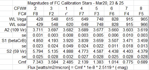
Figure 7. Magnitudes of 3 secondary standard stars
compared with Vega, assumed to be zero for all bands.
Entries are described in the text (next paragraph).
Figure 7 summarizes results of the Vega calibration transfer
observations to three secondary standard stars. The FC#
notations are those defined by the Dawn Framing Camera
experiment team. I have assigned CFW# labels, corresponding to
their sequence in the color filter wheel - which was also
their wavelength sequence. One exception is the r'-band
filter, which I originally intended to use as a "reality
check" but later dropped when I felt that there were no
problems requiring a reality check.
This table shows magnitudes in the invented magnitude system
for each FC filter band. The way to convert a magnitude to
flux is to use the equation at the bottom of the figure. For
example, using the 548 nm filter the flux for 59 Vir is
3.584e-8 × 2.5119^(-5.135 ± 0.028), which is (3.166 ± 0.081) × 1e-10 [watts/m2/micron].
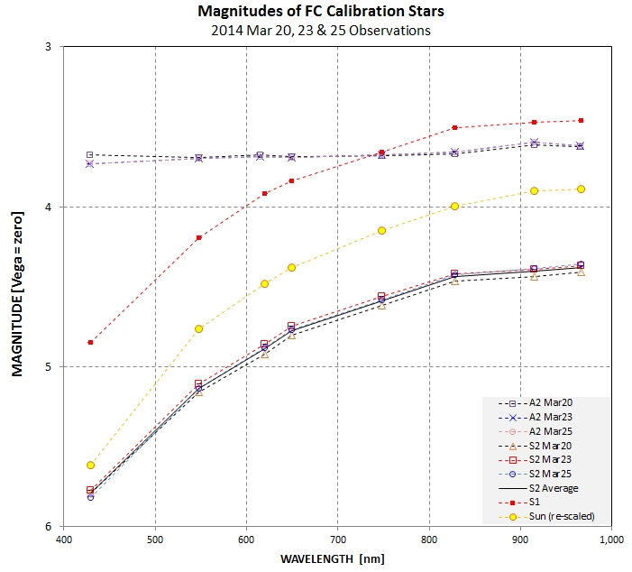
Figure 8. FC magnitudes for secondary calibration
stars from 3 dates, plus the sun's spectrum re-scaled to
appear on the graph. Vega, by definition, has FC
magnitudes that are all zero.
This plot shows that star A2, spectral type A, has magnitudes
versus wavelength, relative to Vega, that are "flat," meaning
that it has the same spectral shape as Vega. This is to be expected. Star
S1, spectral type G0V, is quite different and resembles the
sun's spectral shape. Again, this is to be expected since its
spectral type is similar to the sun's (G2V). Star S2 (59 Vir) has FC
magnitudes versus wavelength that also resemble the sun's in
shape, as expected since Vir 59 has a spectral type of G0V.
The differences in S2 (59 Vir) magnitudes are used to estimate
the uncertainty of the average (plotted as a solid black trace
and listed in Fig. 7). The star S2 (59 Vir) has a flux with an
uncertainty of ~ 2.8 %. This is the largest uncertainty in the
chain of calibration steps leading to geometric albedos for
Vesta and Ceres. Recall that there is a 1.8 % SE associated
with the ratio of collecting area of the 1-inch mask hole to
the unmasked aperture. Combining this with the 2.8 % SE yields
a total SE of 3.3 %. Given that Ceres has a geometric albedo
of ~ 9.6 %, calibration uncertainties will account for a
geometric albedo uncertainty of ~ 0.32 % (e.g., Ag
= 9.60 ± 0.32 %).
By observing either Vesta or Ceres in alternation with 59 Vir,
for example, using techniques described in the next section,
it is possible to determine a ratio for the flux of the
asteroid to 59 Vir, which a simple multiplication by the flux
of 59 Vir yields the flux for the asteroid.
A few subtleties should be
addressed now.
Notice that in Fig. 7 the wavelength
(WL) rows have slightly different values for Vega and "solar."
This is because the slopes of the Vega and solar spectra
differ, and the spectrum-weighted average wavelength is
therefore slightly different for each source.
In deriving fluxes for the secondary calibration stars the
ratio of brightnesses, star/Vega, is multiplied by the
effective flux of Vega. This latter is the filter passband
weighted flux of Vega, where the passband is shown in Fig. 2
and the Vega flux spectrum is shown in Fig. 3. What if the
real filter response function is flawed by a "light leak." For
example, suppose the shortest wavelength FC filter leaks some
light at the longer wavelengths (leaks at shorter wavelengths
won't matter since flux decreases fast on the short wavelength
side). Light leaks are common at levels below ~ 1% for filters
used by amateurs; this engineering problem is difficult to
solve when the wavelength of interest is at one end of the
spectral energy of the target star (and instrument response
function). Therefore, the 428 and 966 nm FC bands are at the
greatest risk of having light leaks. Because of the very
different spectral energy distributions of Vega and the sun
the effective wavelength of either of these filters could be
significantly different for the two sources than was
calculated for the assumption of no light leaks. A light leak
for the 428 nm band, for example, would be influenced more by
solar type stars than Vega, and this would produce an positive
error in the 59 Vir flux (c.f., Fig. 9). This, in turn, would
cause asteroid fluxes to appear greater than they actually
are, which would be interpreted as a higher geometric albedo
than is actually the case. This is something we should be on
the lookout for in the Vesta and Ceres geometric albedo
results.
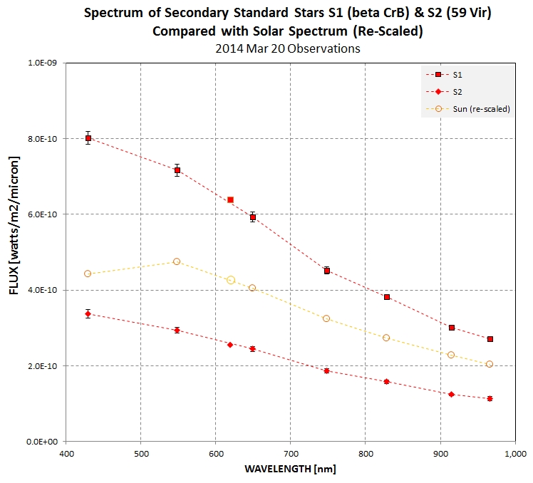
Figure 9. Comparing flux spectra of two sun-like
secondary stars to the sun's spectrum (re-scaled).
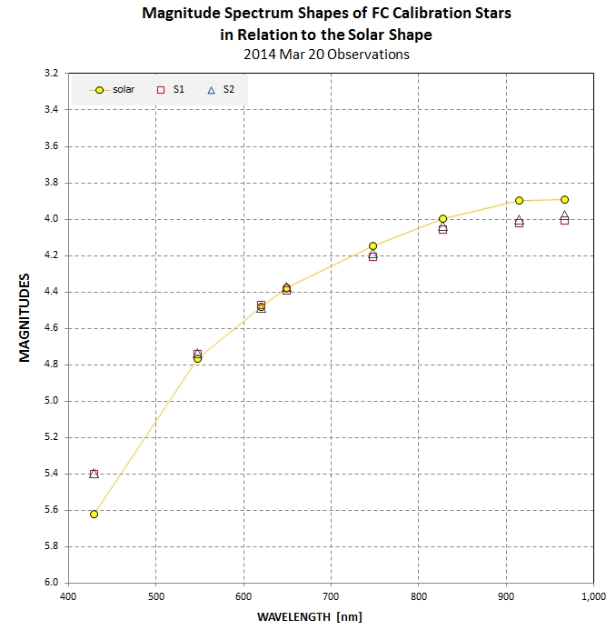
Figure 10. Comparing
shapes of FC spectra for two solar like
stars (G0V) with the sun's FC spectrum (spectral
type G2V), showing
a suspicious "too high" flux for the 429 nm
FC band (consistent with a "light leak" for
that FC filter).
Another subtly is the matter of stellar variability of the
secondary standard stars. "All stars are variables" at some
level, but could 59 Vir, for example, be variable at a level
that would matter for the goal of measuring and monitoring
geometric albedo? In every observing session where 59 Vir and
the other secondary calibration stars were measured on the
same observing session there was no evidence for changes. 59
Vir has a spectral type of G0, so it is unlikely to be
variable.
Phase
2: Transferring Secondary Standard Stars to Vesta and Ceres
The same all-sky procedures used for
transferring Vega fluxes to secondary standard stars, described
in the previous section, were used to transfer fluxes from the
secondary standard stars to Vesta and Ceres. Since Vesta and
Ceres were closer in the sky to the secondary standard stars
this transfer process is expected to have been achieved with
much better accuracy.
In the interest of brevity I'll refer to just one secondary
standard star, S2 (i.e., 59 Vir), even though others were
sometimes also observed, and I'll refer to observing Ceres even
though I often observed Ceres and Vesta during the same
observing session. Since Ceres and S2 were in the same part of
the sky they rose and set together, and had a similar air mass
versus UT in between. This meant that it was possible to
alternate observations of them in a way that assured similar air
mass values, and it also assured that temporal variations of
atmospheric extinction would have negligible effect upon their
flux ratio comparisons. In almost every case I used the odd/even
rule for observing target and reference. For example:
tgt/ref/tgt has an odd number of target observations and an even
number of reference observations, and the average time of their
observations is close to the same and therefore unaffected by
linear trends (of atmospheric extinction, for example). A range
of high air mass to low air mass observing was also planned,
which would allow a more accurate measurement of that observing
session's atmospheric extinction.
The Ceres image set for one FC band (all images for the
night) would be loaded into MaxIm DL for processing. After
calibration (bias, dark and flat) all images would be aligned so
that Ceres was at the same pixel location. An artificial star
would then be inserted in a corner of each image (64x64 image
with Gaussian function having FWHM = 3.77 pixels and peak DN =
65,535 on a field of zeros). A photometry aperture was selected
that assured >99% capture for all (accepted) images. The
photometry tool was used to produce a CSV-file with 3
columns: JD, target magnitude and reference (artificial
star) magnitude (allowed to default to zero for all images). The
same procedure was used to process each secondary calibration
star's image set. All CSV-files were imported to a
spreadsheet template that was designed for this project.
By entering Ceres target RA/DE coordinates, and selecting RA/DE
from a table for the secondary standard stars, the JD values
could be converted to air mass values for each image. The
spreadsheet was used to derive an atmospheric extinction vs. UT
function (details too tedious to describe). I'll just state here
that the Ceres instrumental magnitudes couldn't be used for
deriving extinction because the asteroid changed brightness
during the night; thus, all atmospheric extinction solutions
were performed on the secondary star measurements. Figure 10
illustrates how an extinction model was adjusted (Rayleigh,
aerosols, ozone and water vapor) to match measured average
extinction for an observing session. The theoretical atmospheric
model "guided" a choice for the model of extinction vs. UT for
the observing session.
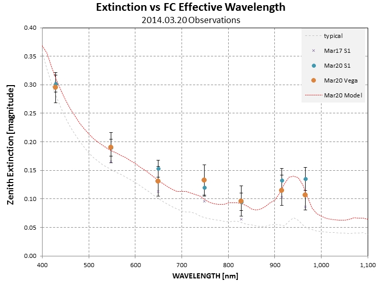
Figure 11. Atmospheric extinction for 7 FC bands for
Vega and S1 on one date, compared with an extinction model.
After settling on a model for extinction vs. UT for a FC
band, Ceres magnitudes were determined by comparing Ceres
instrumental magnitudes with the secondary star instrumental
magnitudes (where each secondary star had a magnitude assigned
to it by the "Vega to secondary star calibration procedure,"
described in the previous section).
The procedure just described was performed for each of the FC
bands, and an archive of Ceres calibrated magnitudes was created
for each observing date in this manner. After each
observing session had been processed to the stage of having
calibrated magnitudes for each FC band an optional next level of
processing was usually performed. This consisted of converting
magnitudes to standard values (the 1,1, or 1 au and 1 au
versions), and fitting them with a HG and rotation model. The
rotation model used phase-folding for an adopted rotation
period, with a small phase shift associated with the Ceres sky
location. On occasions (weeks apart, usually) the standard
magnitudes for all dates (for one FC band) would be copied and
sorted, and a running median was used to establish a new
rotation variation model (for the FC band). This was used to
identify outliers in all previous data, and the non-outlier data
was used to refine the HG model fit. These data were converted
to geometric albedo and plotted as a way of monitoring adequacy
of the accumulated observations. Figure 11 is an example of this
for one FC band.
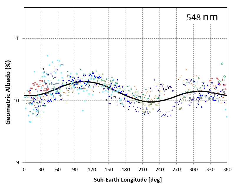
Figure 12. Rotation variation of geometric albedo for
the FC 548 nm band, using a HG model that minimized residuals.
Different symbols are used for different observing session
dates.
At the completion of the Ceres opposition observing season the
magnitudes for all FC bands was converted to fluxes and shared
with team members for additional modeling analysis.
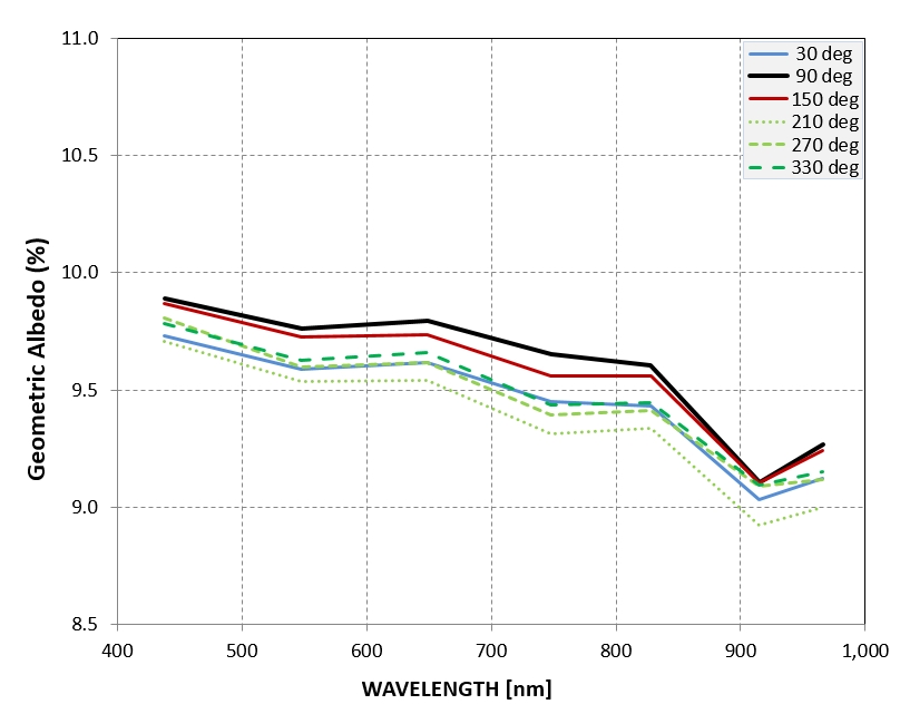
Plots of geometric albedo versus wavelength for a selection
of rotation phases, showing a slight "blueness" color for at
all times. The absorption feature at 920 nm is evident, and
appears to have a different depth with rotation.
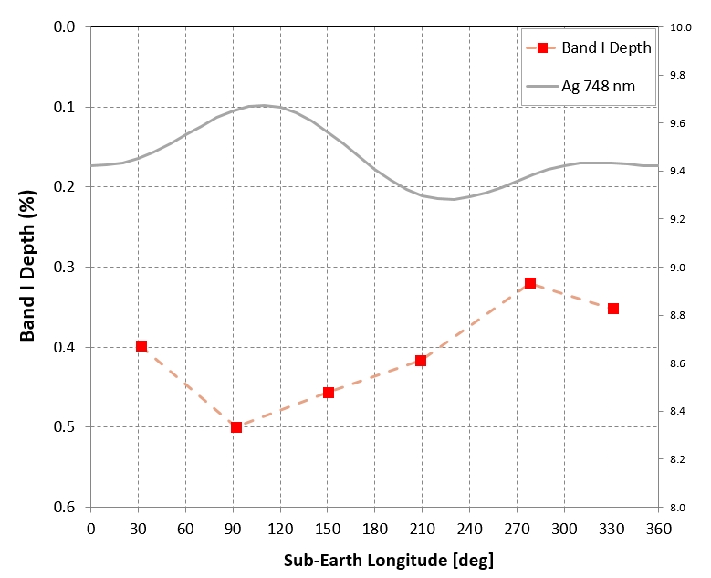
Depth of the absorption feature at 920 nm, Band I, is deepest
at a rotation phase corresponding to sub-Earth
longitude of ~ 90 deg, which is also the rotation phase time
when geometric albedo is maximum.
This last graph can be used to estimate "relative calibration"
uncertainty, or band-to-band calibration SE. I have estimated
that the "absolute calibration" SE is 3.3% for all bands except
the shortest wavelength band (438 nm), where absolute
calibration SE is probably 5%. Some of the uncertainty
components are shared by all bands, such as the 1.8% SE
associated with the aperture mask used to observe Vega for
transfer of its fluxes to the fainter secondary calibration
stars. Therefore, the band-to-band calibration SE is smaller
than the 3.3% and 5% values. It is sometimes difficult to
estimate "relative SE" but we can infer an approximate estimate
"after the fact" by comparing how results are related to each
other with guidance from an understanding of how they "should"
be related to each other if calibration uncertainties didn't
exist. Consider the above graph. If the positive correlation
between geometric albedo and Band I were perfect, for example,
then the small departures from such a correlation would require
errors in geometric albedo on the order of 0.1% (i.e., geometric
albedo for each measurement ~ 9.5 ± 0.1%). If, on the other
hand, the geometric albedos were subject to random errors
greater than 0.1%, how could the correlation pattern in the
above graph exist? If the position is taken that there is no
relationship between Band I depth and geometric albedo then the
scatter of Band I depth values about an average implies that
individual albedo determinations have srrors of ~ 0.03% (i.e.,
geometric albedo ~ 9.5 ± 0.3%). This would be
the most conservative interpretation of the above graph, so
I conclude by suggesting that whereas the absolute
calibration SE for geometric albedos for wavelengths longer
than 500 nm is 3.3%, their band-to-band relative SE is ~
0.3%. Stochastic SE for other graphs of geometric albedo
will of course be an orthogonal sum of the 0.3% band-to-band
albedo SE with the appropriate stochastic albedo component.
A summary of results of my analysis of these
data can be found at: http://brucegary.net/Dawn/Ceres.html
Lessons Learned
The most important uncertainty in the calibration process came
from the transfer of Vega fluxes to a secondary standard star.
This 2.8% uncertainty is greater than the 1.8% uncertainty
associated with measuring the ratio of collecting area for the
1-inch hole mask and the unmasked aperture. If I
were to do this project over I'd devote more observing
sessions to the task of transferring Vega
flux to a secondary standard star.
The APASS BVg'r'i' magnitudes exhibit an internal consistency of
~ 10 mmag for most star fields. It is estimated that the
accuracy of the g'r'i' magnitudes is somewhere in the 1 to 2 %
region (reference needed; ask Arne). If it's 1.5 % then this is
twice as good as what I achieved. This means that a more
accurate determination of the Ceres geometric albedo spectrum
could be achieved by observing with SDSS filters. Since the FC
filters response functions are narrower than those for the SDSS
filters there would be a loss of spectral resolution, but this
would only be important where spectral structure exists - such
as Vesta's Band I region. There appears to be almost no
structure in the Ceres spectrum, so SDSS filters should be free
of any spectral resolution loss. I therefore recommend that any
future attempt to improve the FC calibration be performed using
SDSS filters.
Data File
Ceres data file of fluxes: link
References
Kurucz, R. L., 2003, Index of Stars: Vega, http://kurucz.harvard.edu/stars/vega
2000 ASTM Standard Extraterrestrial Spectrum Reference E-490-00:
http://rredc.nrel.gov/solar/spectra/am0/ASTM2000.html
________________________________________________________________
This site opened: 2015.01.12 by Bruce L. Gary (B L G A R Y at u m i c h dot e d
u).