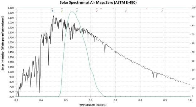
Figure 2. Solar spectrum for the wavelength region where CCD cameras respond, showing spectral location of a standard filter (V).
This web page describes some basic concepts required for the creation of a new magnitude system, specifically intended as support for the Dawn Framing Camera 7-band magnitude system that I created for calibrating Vesta and Ceres geometric albedo in 2014 (link).
Deriving
a Magnitude
System
Bruce
Gary, 2014.03.10
Introduction
When using a filter
that does not
belong to one of the standard filter bands it is important to
characterize
measurements made with it in terms that relate to physical
phenomena, such as energy
flux [watts per m2 per micron]. If this can be
accomplished then
measurements with the new filter can be used to fill gaps in the
“spectral
energy distribution” (SED) spectrum of stars. In addition, such
measurements
can be used to add detail to an asteroid’s albedo. This write-up
describes an
invention of a new magnitude system using a standard filter as a
test case,
which can serve as a model for doing the same for other filters
(such as the
Dawn FC filters). The underlying philosophy for a magnitude system
is that any
observer who processes his observations properly can state that
his magnitude
is what would have been measured by the telescope system used to
create the
magnitude system, and that such magnitude can be converted to a
physically useful
property such as flux at an effective wavelength.
Solar Spectrum
The sun’s spectrum
is shown in
Figures 1 and 2.
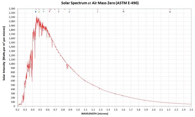
Figure 2. Solar
spectrum for
the wavelength region where CCD cameras respond, showing
spectral location of a
standard filter (V).
The solar energy
spectrum is
approximately constant across V-band. The effective width of the
V-band shape
is ~ 0.10 micron, and the average solar flux within this region is
~ 1850
[watts/m2/micron]. (Note my use of “watts/m2/micron”
to
be the same as “watts per m2 per micron.”) Therefore, a
V-band
filter above the atmosphere would transmit ~ 185 [watts/m2].
How many photons is
that? Well,
the energy of a 0.55 micron photon is hν,
where h is Planck’s
constant and ν
(frequency) is c/λ (c is speed of light). A 0.55 micron photon has
an energy of
3.61e-19 [watts]. Therefore, 185 [watts/m2] within the
V-band
corresponds to 5.12e+20 photons per second per m2. At
other
wavelengths photon energy will differ: energy/photon = 5.12e+20 ×
0.55 /
λ[micron]. This information allows us to convert Fig. 2 to a plot
of photon
flux, shown as Fig. 3.
Using Fig. 3, and
noting that
V-band is ~0.1 micron wide, we can estimate that a V-band filter
above the
atmosphere would transmit ~5e+20 [photons per second per m2].
This
agrees with the previous estimate.
For wideband
filters, such as a
clear filter, it is appropriate to work with photon flux spectra
since a CCD
camera produces data numbers (DN) proportional to the number of
photons intercepted
by pixels and available for conversion to photo-electrons; in
other words, DN
is not proportional to “energy per unit are per unit wavelength”
and using an
energy spectrum would be misleading. It is common practice to
convert an
“energy per unit area per unit wavelength” spectrum, referred to
as Fλ,
to something proportional to “photons per unit area per unit
wavelength” by
simply multiplying Fλ by λ, yielding λFλ
[watts/m2].
Such a spectrum will have the same shape as Fig. 3, and will be
proportional to
“photons per unit area per unit wavelength” but the invented
parameter has a
difficult to understand meaning and the units are meaningless to
me (since the
“per micron” unit is missing, yet is implicit in λFλ).
For filters
with narrow pass-bands it will be acceptable to use the “energy
per unit area
per unit wavelength” spectrum (e.g., Fig. 2), so that’s what I
will do in the
remainder of this document.
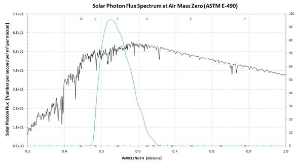
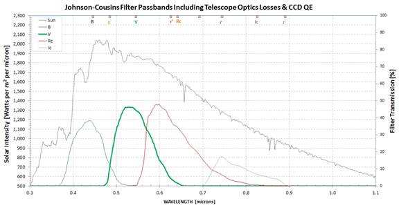
Fig. 4 shows the
effect of
hardware on filter pass-bands; the response loss is due to
telescope optical
transmission and CCD QE response.
In creating a new
magnitude
system it is necessary to use the pass-band response functions of
the entire
telescope hardware system: telescope optical transmission, filter
response and
CCD QE. After all, if the system that uses a filter doesn’t
respond to a
wavelength region then nothing related to that region should enter
into
consideration of a magnitude system for that filter band. This has
been true
for the calibrations of the BVRcIc and u’g’r’i’z’ standards.
Atmospheric extinction requires a different treatment from the hardware losses and responses. Extinction effects must be removed before any magnitude determinations can be made. In effect, we are asking what the standard telescope system would observe if it were above the atmosphere, and anyone else who wants to use the magnitude system must do the same. Since each observer will have a different telescope system spectral response a method has to be devised for converting an observer’s measurement to an equivalent of what the standard telescope system would have observed (above the atmosphere). Atmospheric extinction consists of four principle components: Rayleigh scattering, aerosol scattering and absorption, ozone absorption and water vapor absorption. This is shown in the next figure.
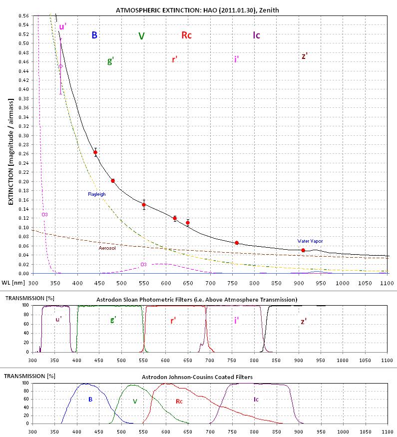
Figure 5. Atmospheric
extinction
at zenith [magnitude] at my observing site on a typical winter
night.
Converting measured
magnitude to
“above the atmosphere magnitude” is straightforward, and will not
be described
here. Instead, I will assume that all measurements will be
converted to above
the atmosphere magnitudes before any attempt is made to convert an
“instrumental magnitude” to a standard magnitude. (Details may be
given later.)
Referring back to
Fig. 4, notice
that a V-band filter for my telescope system responds to photons
between 480
and 640 nm, and the effective wavelength for this filter response
function is
546 nm (detailed calculation takes into account that CCD responds
to photons). The
“filter response weighted solar flux” is 1853 [watts/m2/micron].
If
we want to devise a magnitude system for this filter response
function then
1853 [watts/m2/micron] can play an important part in
such a
creation. For example, if an object was measured to be 1% as
bright as the sun,
5 magnitudes (by definition), we could state that it’s “filter
response
weighted flux” was 18.53 [watts/m2/micron]. Another way
of
expressing this is to state that:
“Star
flux at 546 nm” = 1853 [watts/m2/micron] / 2.5119delta-magnitude
where
“delta-magnitude =
magnitude of unknown target – magnitude of sun.” If we arbitrarily
adopt a magnitude
for the sun then we will have established a new magnitude scale.
However, it is
impractical for any observer to use the sun as a reference
standard, so another
choice should be adopted for a non-variable star to be the
reference.
Vega has
traditionally been used
to establish magnitude scales, and I will do the same. I will
define magnitudes
such that Vega has a zero magnitude for every filter (referenced
to above the
atmosphere).
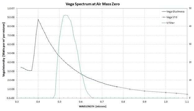
This energy spectrum
for Vega is
well-established. Convolving my V-band response function with the
Vega spectrum
shows that if my telescope were above the atmosphere it would
measure a flux of
3.5e-8 [watts/m2/micron] at an effective wavelength of
0.541 micron.
(This effective wavelength is different from the one given above
due to Vega
being bluer than the sun.) Measurements of any other star (having
the same
blueness as Vega) could then be converted to flux at the same
effective wavelength
using a standard magnitude equation.
“Star
flux at 541 nm” = 3.66e-8 [watts/m2/micron] / 2.5119magnitude
(1)
For this magnitude
system to be
useful a network of stars should be calibrated using Vega as a
primary
standard. Whenever filters are used that have response widths as
large as
V-band, for example, it is necessary to correct for star color
effects. This
means that it is important to establish magnitude scales at other
effective
wavelengths (preferably surrounding the wavelength of greatest
interest), and
to establish calibrated magnitudes for these other bands for stars
having
colors different from Vega.
As a check on the
above, let’s
calculate the sun’s flux at V-band. Since the sun’s V-mag = -26.75
we have
“sun’s flux at 541 nm” = 3.66e-8 / 2.5119-26.75 = 1837
[watts/m2/micron].
This differs by < 1.0% from the 1853 [watts/m2/micron]
value
determined above.
The above procedure
can be
applied to any non-standard filter for the purpose of determining
an object’s
flux in useful physical units, e.g., [watts/m2/micron].
For the task
of measuring asteroid albedo this capability is useful; since we
know the flux
incident upon an asteroid (since we know the sun’s spectrum), the
reflected
flux can be used to determine albedo.
Demonstration of Asteroid Albedo Calculation
Suppose that on
2014.01.28 I
observed Vesta and found V = 7.28 (the ephemeris value). On this
date the
sun-Vesta distance was 2.288 a.u., the Earth-Vesta distance was
1.869 a.u. and
the “phase angle” α (same as STO, sun-target-observer) was 25
degrees. I’ll assume
Vesta has a radius of 260 ± 5 km. Suppose surface roughness is
sufficient to reflect
light in a manner that is 90% of the way between uniform and
Lambertian (for
which disk average = 2/3 of flat disk reflection, for α = 0). I’ll
define a
parameter for this, and give it the value 0.90 ± 0.10. Let’s
assume a phase
function slope (beyond 7 degrees α) = 0.035 ± 0.010
[magnitude/degree].
Combining these assumptions yields an albedo of 15 ± 4 %. I don’t
know enough
about albedos to know if this is reasonable (if it’s a Bond
albedo, or
geometric albedo, etc.) so I’ll simply take the position for now
that the
magnitudes and fluxes derived from my invented magnitude scales
will be useable
by someone knowledgeable in how to use them.
Specific Plan for Calibration of FC Filters
The previous
material
demonstrates a method for creating a magnitude system that has
physical
significance, which for example can be used to assess an
asteroid’s albedo from
ground-based measurements (if its size is known, and other
assumptions are
made). Implementing such a procedure using specific hardware is
definitely
feasible, but it not trivial. It will require some skills that few
professionals are practiced in; namely, all-sky photometry
calibration.
Fortunately I’ve been doing all-sky photometry for ~ 8 years.
The first task will
be to
transfer the magnitude of Vega to a fainter star, such as one at 6th
magnitude. This will require using an aperture mask because Vega
would saturate
my CCD at all bands using a full aperture. Any fainter stars with
transferred
magnitudes, using the new magnitude systems, will be secondary
standards, while
Vega will be my primary standard. The secondary standard stars
will be located
in the vicinity of Ceres during its 2014 opposition, RA/DE =
13:52+03. The star
83-Tau Virginis is a mere 3 degrees away from Ceres at opposition
(Mar 20), and
it’s a main sequence star with a similar spectral type to Vega (A3
vs A0).
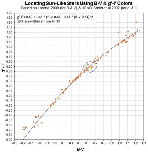
Sun-like stars will also be important to include in the secondary
standard list
because I’ll need to verify the accuracy of star color
corrections. The shape
of flux vs wavelength for the sun-like secondary standards should
resemble the
solar flux spectrum, so this can serve as an internal consistency
check. I’ve
already identified a half dozen sunlike stars near the Ceres
opposition
location, using the criteria B-V and g’-i’ colors must both be
within 0.05 mag
of the sun’s colors. Fig. 7 is a color/color scatter plot showing
that ~ 13% of
stars meet this criterion.
A second task, which
can be done
in parallel with the first one, is to calculate pass-band shapes
for my
hardware and then calculate the fluxes that each filter would
intercept from
Vega (above the atmosphere) for conversion to photo-electrons.
This will permit
the creation of a set of equations, one for each filter i
(analogous to eqn.
(1), above):
Star
flux [watts/m2/micron] = Ci / 2.5119 magnitude
(2)
Another check for
the Ci
coefficients will be to compare SEDs (spectral energy
distributions) for the
secondary sun-like stars with their known BVRcIc and u’g’r’i’z’
SEDs. The SED
spectrum derived from eqn (2) should overlap with the SED from
known magnitudes
(APASS, etc). When this can be demonstrated then it is likely that
any
measurements of Ceres, or any asteroid, using the eqn (2) Ci
set and
the FC filters should be correct.
This site opened: 2015.01.14 by Bruce L. Gary (B L G A R Y at u m i c h dot e d u).