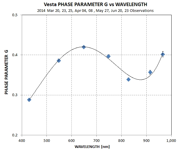
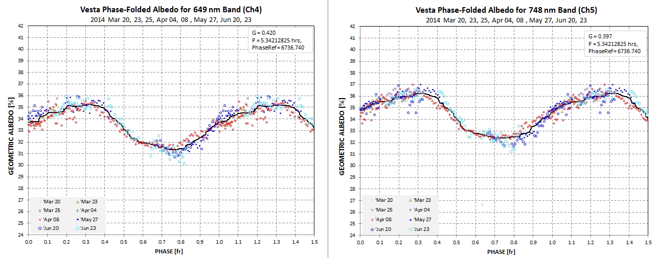
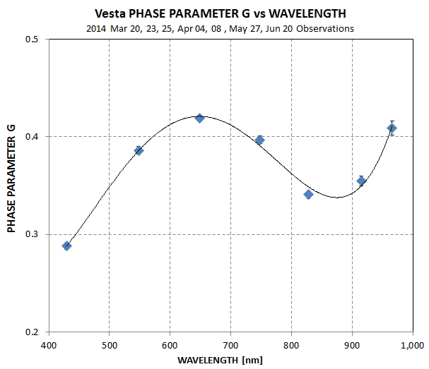
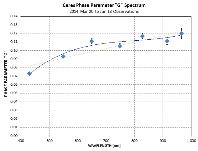
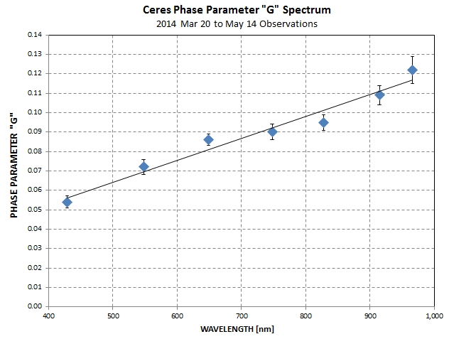
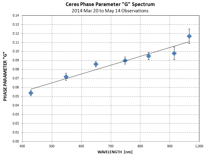
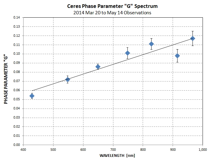
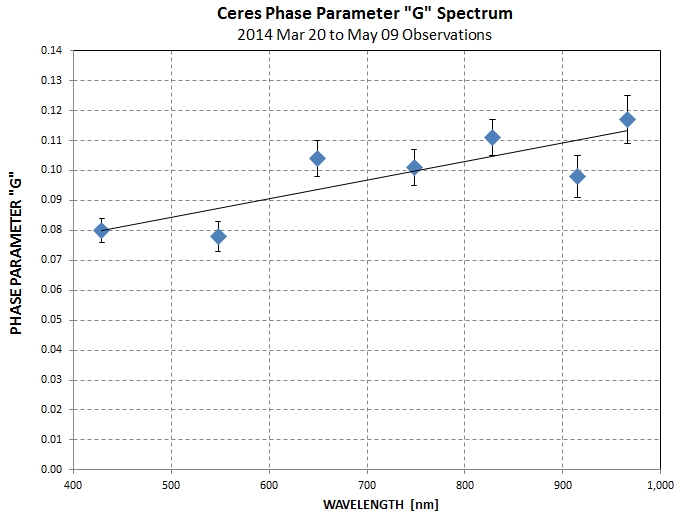
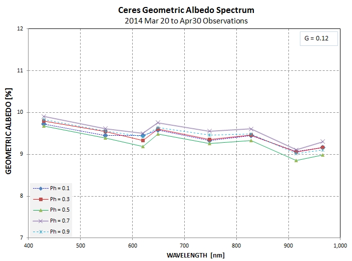

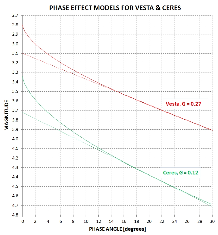
2014.04.10. Decided to adopt the phase effect given by the HG equations and G values shown on the plot below.
2014.04.10. More bands for Vesta albedo vs rotation phase. A better presentation of all Vesta data, summarized, can be found at the Vesta Summary web page (linked above). All Vesta geometric albedos in the graphs below will be adjusted downward by ~ 2% after I implement a revised phase effect model (using G = 0.28). [Note: the plots for this date have been superseded by ones located in the Vesta summary web page.]
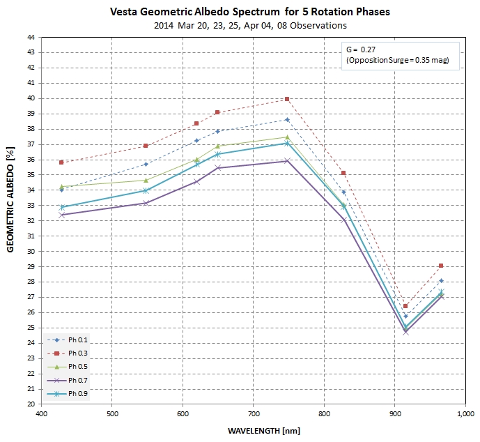
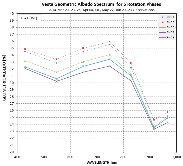
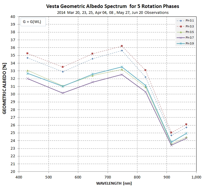
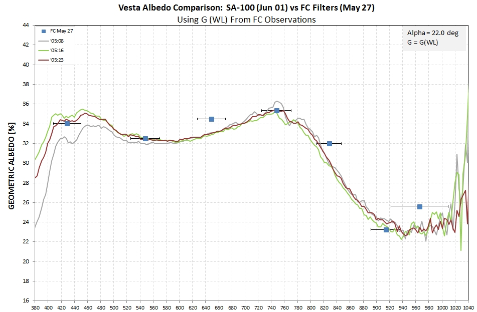
Summary of Vesta albedo vs wavelength for 5 rotation phases.
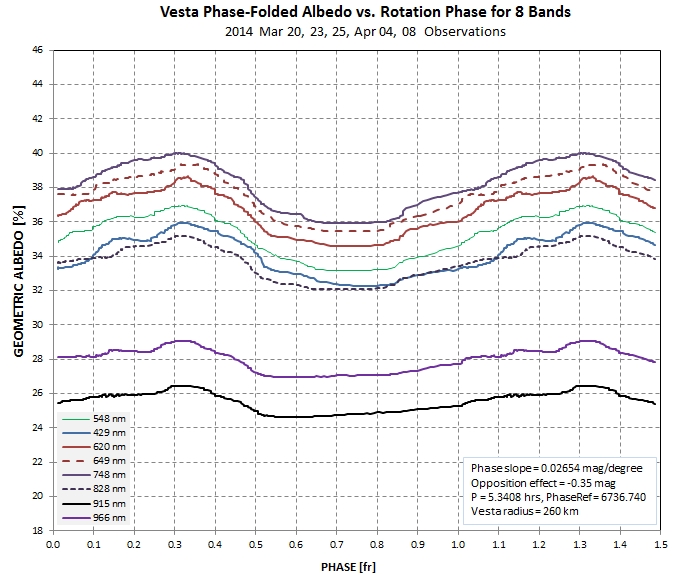
Summary of Vesta albedo vs. rotation phase for 8 bands.
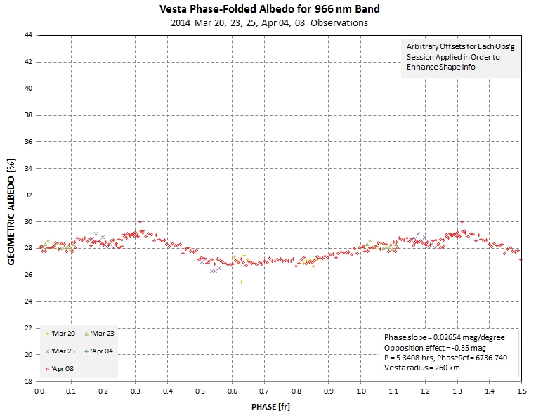
Vesta albedo at 966 nm for 5 observing sessions.
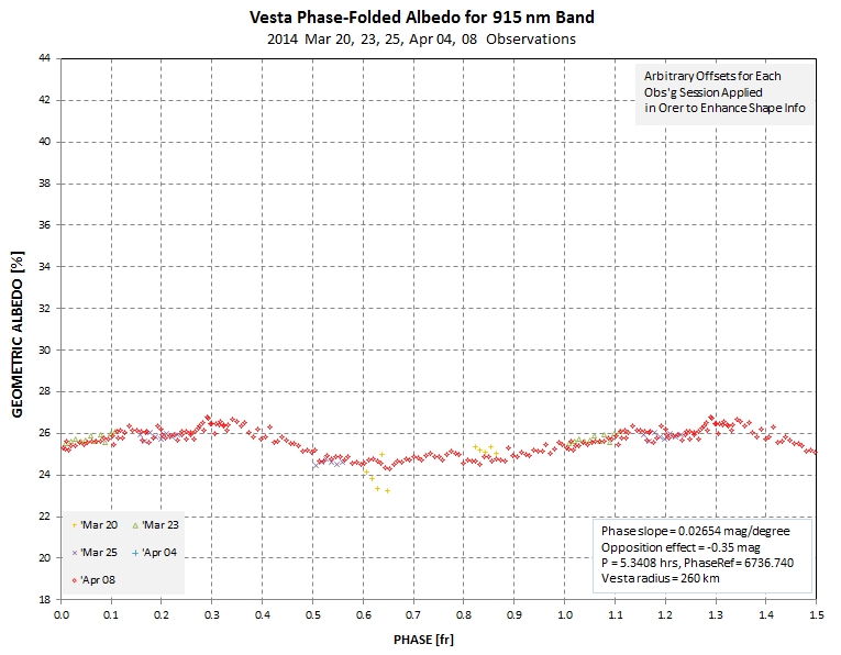
Vesta albedo at 915 nm for 5 observing sessions.
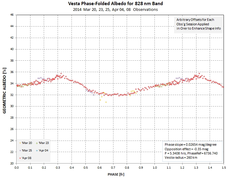
Vesta albedo at 828 nm for 5 observing sessions.
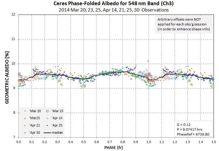
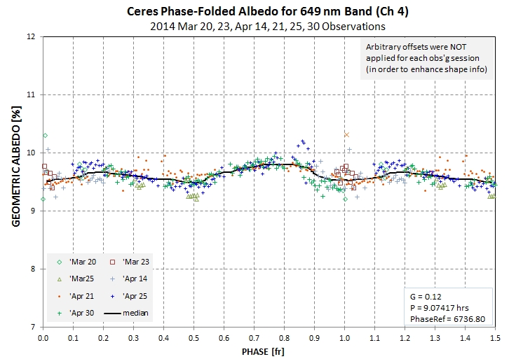
2014.04.09. Here's a Vesta albedo vs. rotation phase for the 548, 649 & 748 nm bands. They are less noisy than the 429 nm band data due to lower atmospheric extinction and lower levels of systematic errors due to extinction trend corrections.
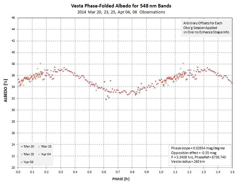
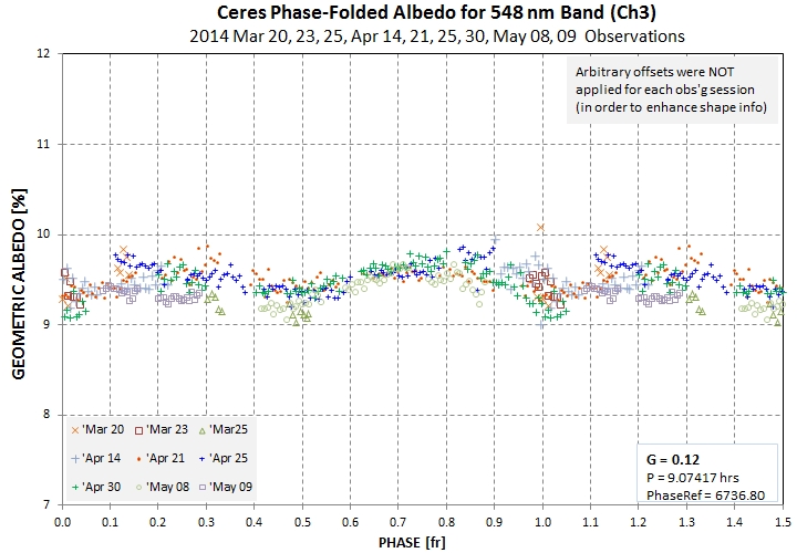
Albedo at 548 nm for 5 observing sessions.
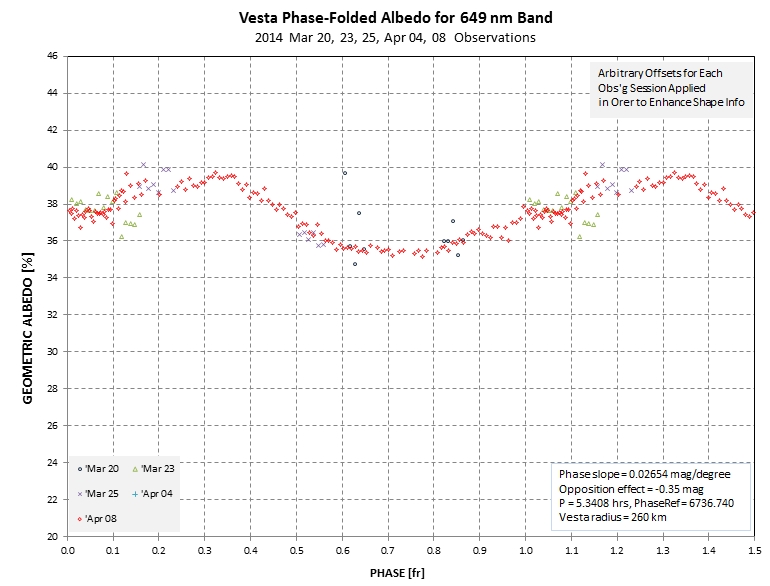
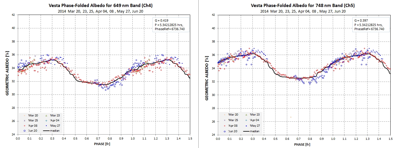
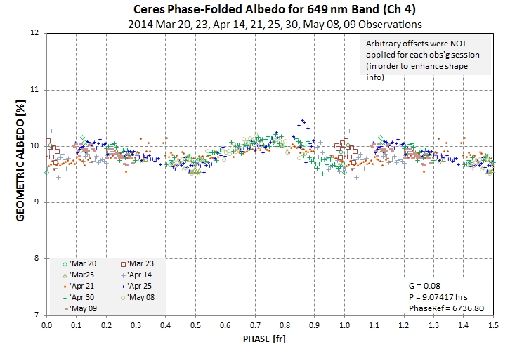
Albedo at 649 nm for 5 observing sessions.
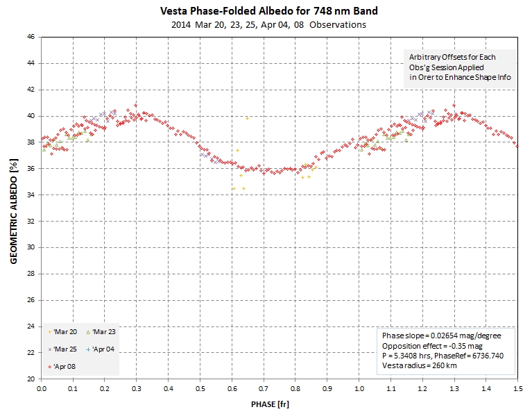
Albedo at 748 nm for 5 observing sessions.
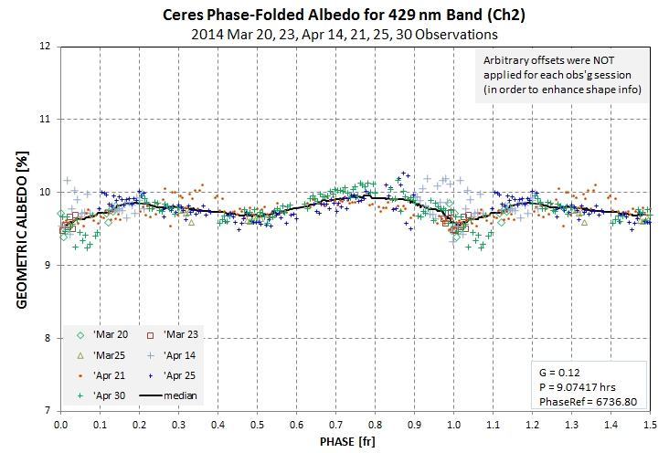
2014.04.08. Obs'd Vesta all night last night (1.3 rotations), & have processed Ch2. A significant temporal trend in extinction required that I incorporate a trend term in the spreadsheet analysis. In order to obtain shape information for a plot of albedo vs. phase I created a graph that employs arbitrary offsets (averaging 0.1 ± 0.9 %) that are applied to each observing session.
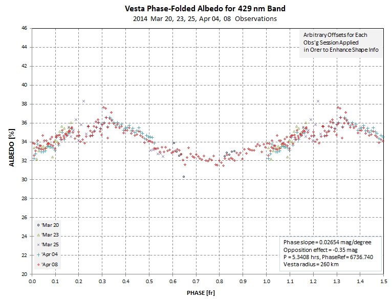
Albedo at 429 nm for 5 observing sessions.
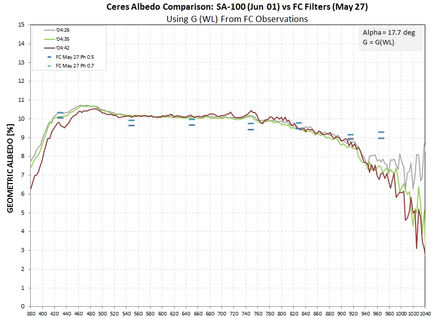
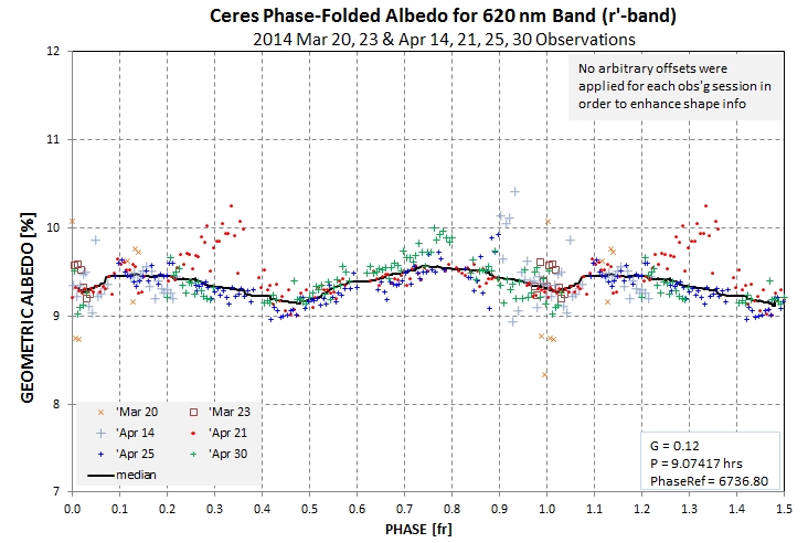
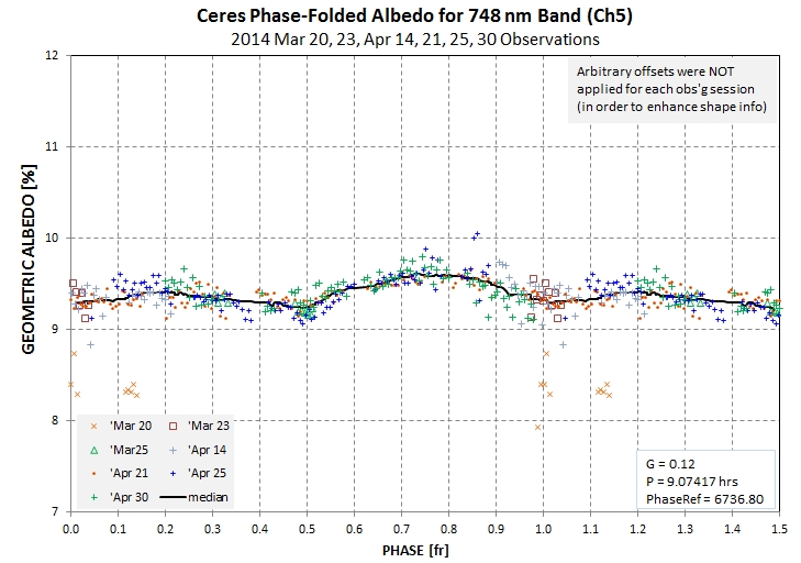
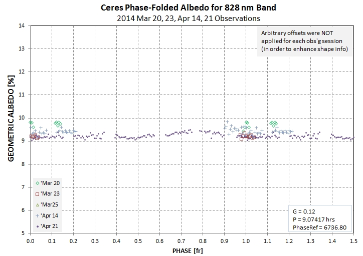
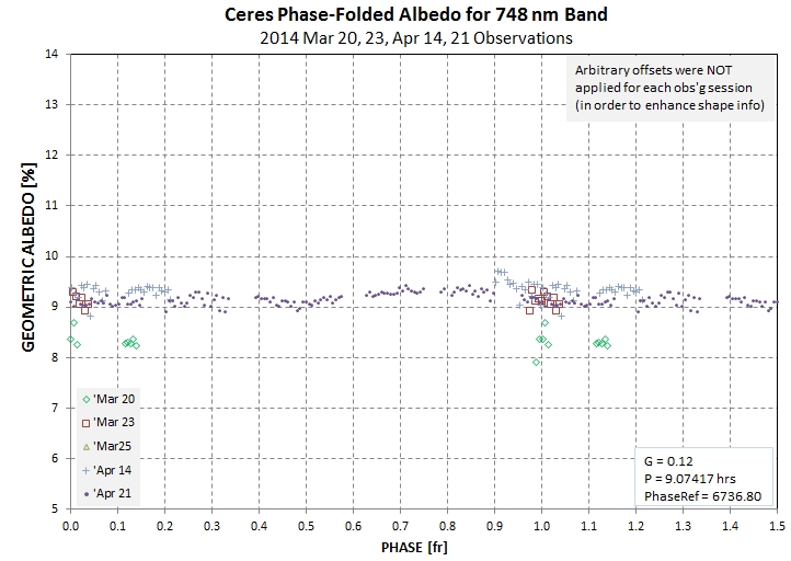
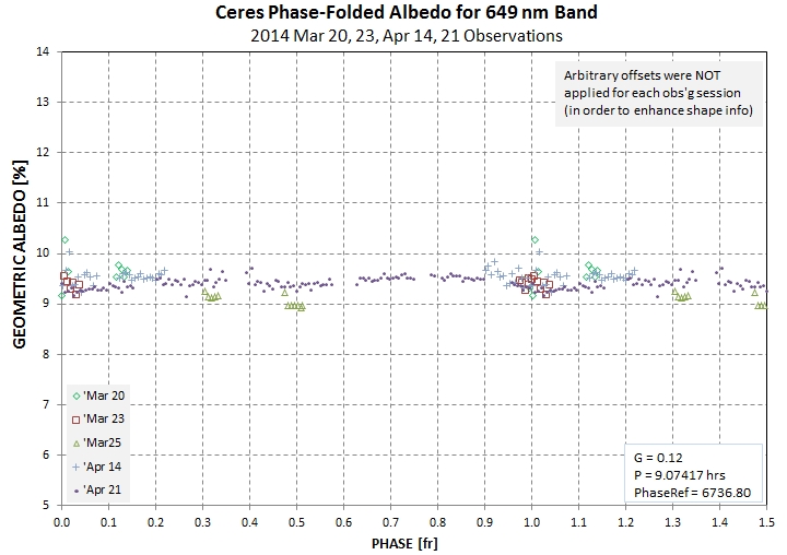
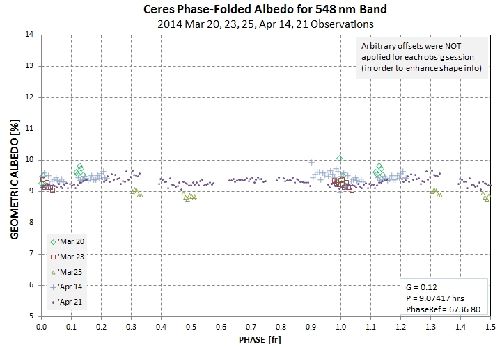
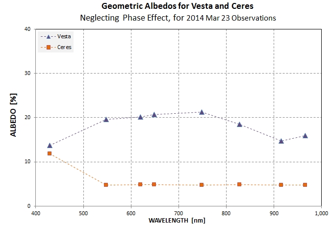
2014.04.07. Added Ceres albedo result for Mar 23 image set. I don't know if the differences are real until we get more data on phase-folded light curve. The 748 nm "dip" feature is not present in the Mar 23 data, so I suspect the dip is not real (I double-checked analysis for it & couldn't find an error).
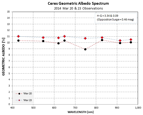
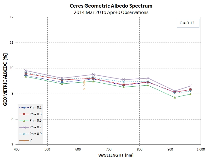
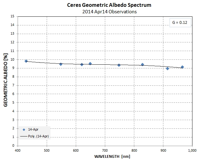
Geometric albedo spectrum for one phase (Mar 20 & 23), made at different dates & phases.
2014.04.06. I've begun processing Ceres data (available for Mar 20, 23 & 25). I've adopted a G value of 0.09 (which ~ doubles flux for phase of 12 deg). This G value is uncertain, ranging from 0.05 to 0.12 in the literature, so I chose an average value.
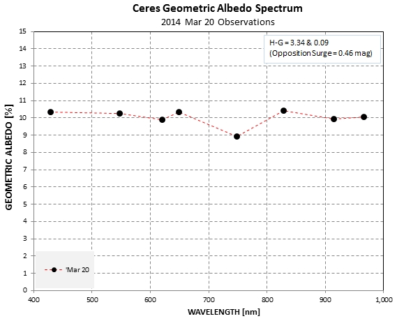
Geometric albedo spectrum for one phase (Mar 20).
2014.04.05. Changed adopted Vesta radius to 260 km (from 265 km) & replotted geometric albedos.
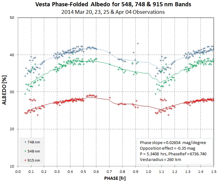
All geometric albedo measurements for 3 bands and smoothed version (median running filter).
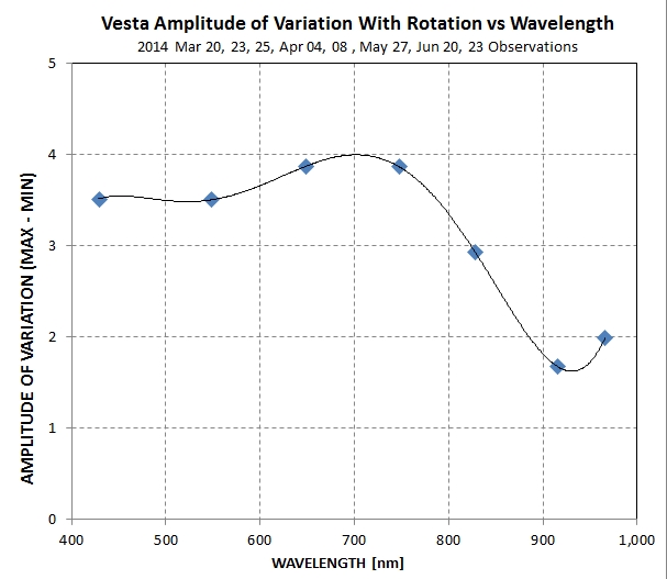
2014.04.04. Obs'd last night, 5 hrs; first session emphasizing asteroids (vs. calibrating secondary stars). Processed S2 and Vesta image sets. Data are generally compatible with previous (sparse) data. Amplitude of variation with rotation is ~ 0.2 mag.
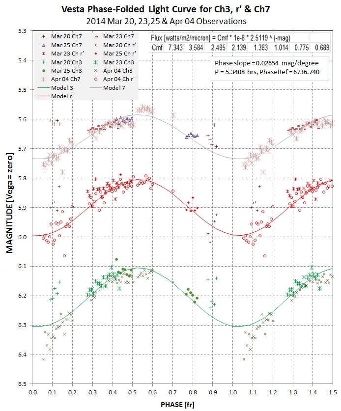
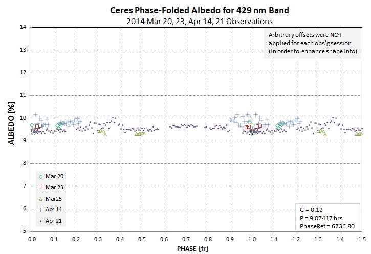
Phase-folded rotation light curve for 3 of the 8 bands available from 4 observing sessions.
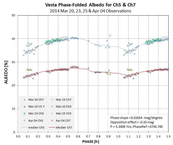
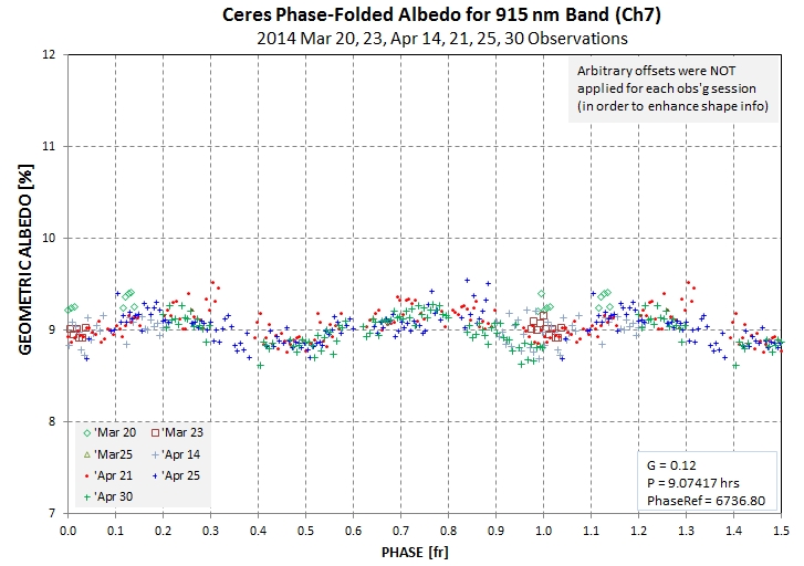
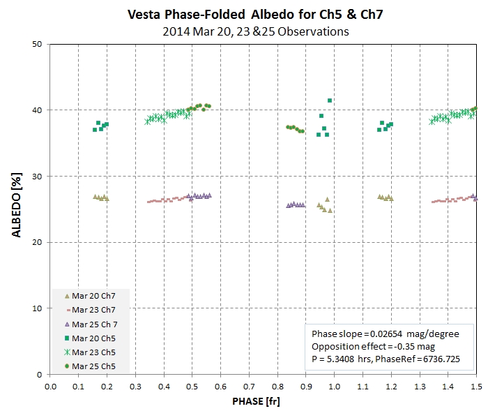
Geometric albedo for Ch 5 & 7 (748 & 915 nm) vs. phase for 4 observing sessions.
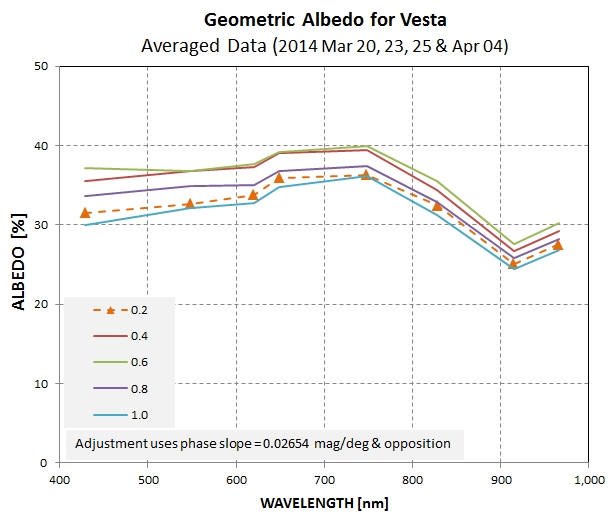
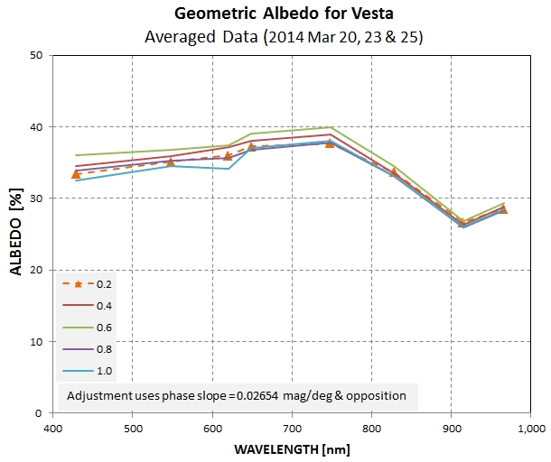
Data is binned by rotation phase and averaged, then plotted vs. wavelength.
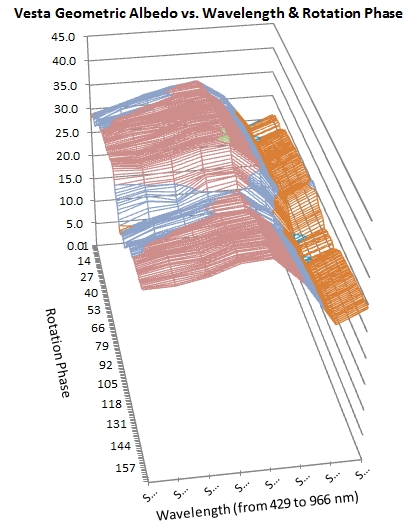
All Vesta albedo data has been smoothed and plotted vs rotation phase and wavelength.
2014.04.03. Here are another two ways to plot Vesta albedo vs wavelength & rotation.
Data is binned by rotation phase and averaged, then plotted vs. wavelength.
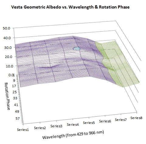
All Vesta albedo data has been smoothed and plotted vs rotation phase and wavelength.
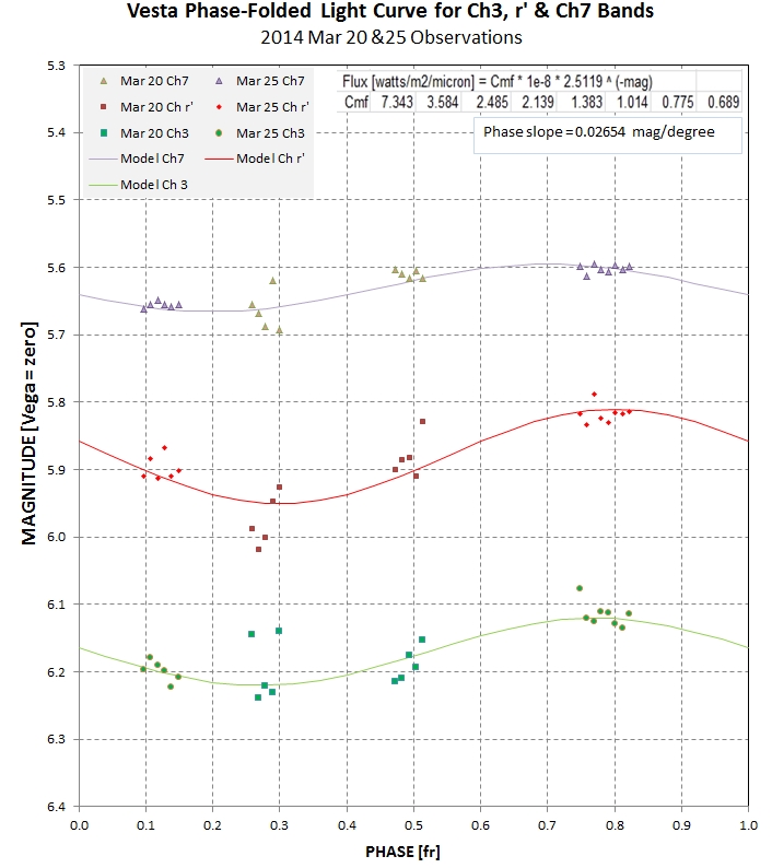
2014.04.02. Determined rotation period to be 5.3408 ± 0.0010 hours, based on Jan 28 and Mar 20,23,25 comparison (corrected for STO change). Below is a plot of Vesta magnitude vs. rotation phase for a sampling of bands.
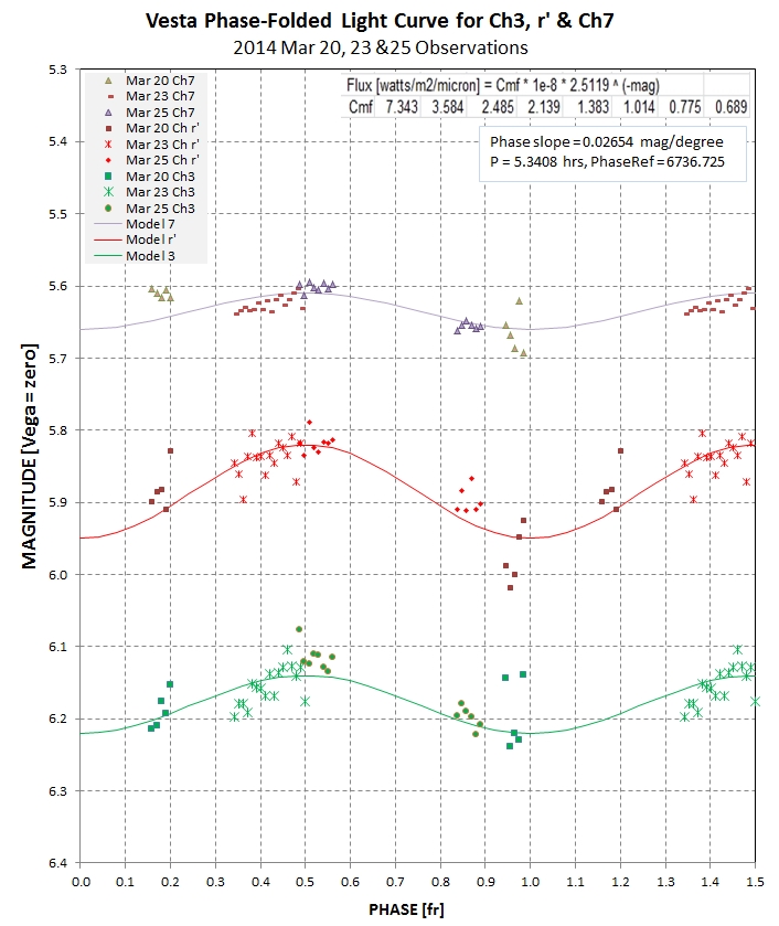
Revised phase-folded rotation light curve for 3 of the 8 bands available from 3 observing sessions.
The next plot shows albedo vs. rotation phase for two bands (the first 5 data, from Mar 20, Ch 5, at rotation phase ~0.95, are noisy due to high airmass scintillation).
Geometric albedo for Ch 5 & 7 (748 & 915 nm) vs. phase.
2014.04.01. Added Mar 23 Vesta data to phase-fold rotation plot.
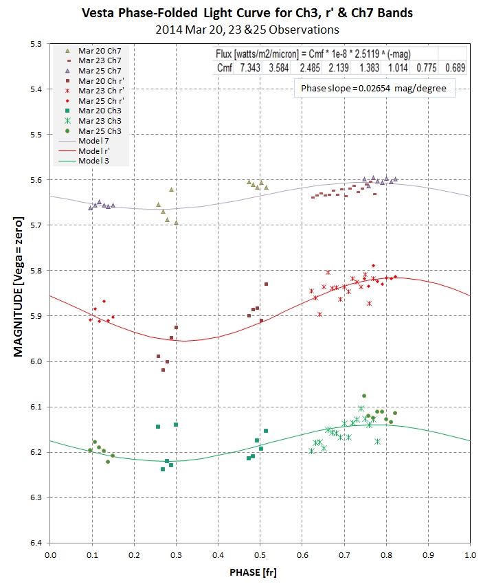
Phase-folded rotation light curve for 3 of the 8 bands available, for all 3 observing sessions available to date.
2014.03.31. Processed Vesta obsn's for a 2nd date; created phase-folded rotation LC showing magnitude for 3 bands. This is just the beginning of phase-fold analysis because observing emphasis until now has been for transferring calibration from Vega to the secondary standards with lower priority for Vesta and Ceres observations. From now on the observations will emphasize Vesta and Ceres, using S2 as a calibration star.
Phase-folded rotation light curve for 3 of the 8 bands available.
Adjusted Vesta geometric albedo for phase effect, using phase slope of 0.02654 and opposition effect of 0.35 magnitude.
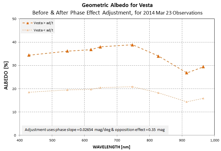
Vesta geometric albedo before & after correcting for phase (using phase slope = +0.02654 magnitude/degree and opposition effect of 0.35 magnitude).
2014.03.30. Below is a Vesta "light curve" for Mar 25.
Vesta light curve for Mar 25, for 8 bands.
2014.03.27. I've finished processing all S1 & S2 image sets (2 & 3 dates). The RMS scatter of 1.9 & 2.6% implies a SE of 1.3% & 1.8% on the averages. Star A2 has a scatter of 1.0%, implying a SE of 0.7% for the average of 3 spectra. Each star can serve as a calibration standard for Vesta and Ceres observations. This concludes my transfer of calibration from Vega to 3 stars near the Vesta/Ceres part of the sky. Any one of these 3 secondary standard stars can be used to achieve acceptable calibration for an observing session of Vesta/Ceres.
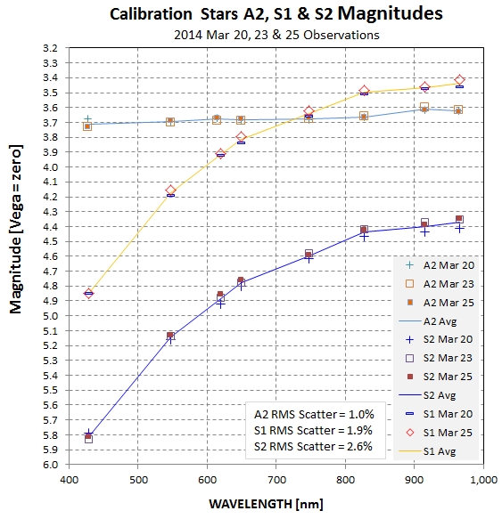
Magnitudes of secondary standard stars A2, S1 and S2 (near Vesta & Ceres), based on Vega being zero magnitude for 3 observing sessions.
2014.03.26. Processed Mar 25 obsns of Vega & A2 (109 Vir), and was pleased to learn that A2 fluxes for the 3 obseravation dates (Mar 20, 23 & 25) exhibit an RMS scatter of 1.0%.
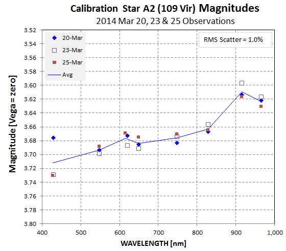
Magnitudes of secondary calibration star A2 (109 Vir) based on transfer from Vega as a zero magnitude primary standard.
Because of the magnitude agreement on 3 dates for star A2 it can serve as a standard for its part of the sky (near Vesta and Ceres). It will therefore no longer be necessary to observe Vega (much later in the morning sky) to provide calibration of Vesta and Ceres observations. Stars S1 and S2 calibrations have not been completed so I don't know if they can also be used for providing calibrations in the Vesta/Ceres part of the sky. They're next on my processing agenda.
2014.03.25. Obs'd all last night: S1, S2, A2, Vega, Ceres, Vesta. Processed rest of Mar 23 data (Vesta & Ceres).
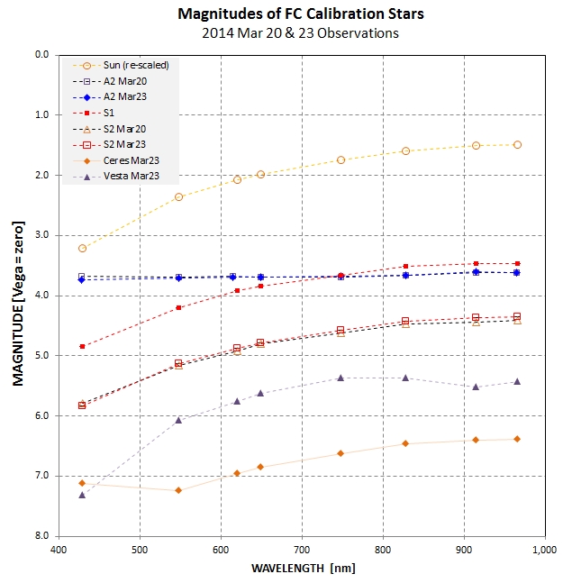
Magnitudes (Vega defined = zero) for 3 secondary calibration stars (Mar 20 & 23) and Vesta and Ceres (Mar23).
Comparing the Vesta and Ceres fluxes (from their magnitudes) enables calculation of albedo. Since I'm not prepared to apply a phase effect adjustment these really aren't "geometric" albedo, but they would be if phase were zero. Since the Vesta and Ceres phases angles are 12 and 11 degrees, we can expect my albedos to be less than the geometric values.
"Albedo" for Vesta and Ceres, defined as measured flux divided by Lambertian flux from flat disk (with diameters of Vesta and Ceres) and facing the sun. In other words, I've ignored changes in brightness with phase angle. The geometric albedo will therefore be slightly greater.
2014.03.24. Temporary hold on processing Mar 20 Ceres & Vesta data in order to process Mar 23 cal star data (Vega, A2 & S2). Below is a plot of the Mar 20 & 23 magnitudes for all secondary standard stars. The A2 overlap is good, whereas the S2 overlap is mediocre.
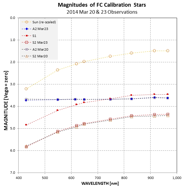
FC Secondary Calibration star magnitudes (Vega defined = zero) for both Mar 20 & 23.
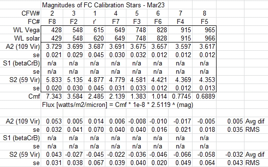
Table of FC Secondary Calibration star magnitudes for Mar 23. The equation for converting magnitude to flux is given. Comparisons of Mar 20 and 23 mag's are given in the bottom section.
Caption correction: Flux [watts/m2/um] = Cmf * 1e-8 * 2.5119 ^ (-mag).
The differences between the Mar 20 & 23 magnitudes for A2 average 0.005 magnitude, with a RMS per filter band of 0.035 magnitude. This is satisfactory.
The differences between the Mar 20 & 23 magnitudes for S2 average 0.032 magnitude, with a RMS per filter band of 0.043 magnitude. This is not satisfactory. A third observing session is needed, and it will emphasize removal of temporal extinction trends (by observing Vega and S2 when both are high in the sky and can be observed close together in time).
2014.03.23. Almost done processing Mar 20 data. Obs'd last night (Vega, A2, S2, Ceres, Vesta); will take 3 or 4 days to process. I determined a more accurate magnitude conversions for the two aperture mask holes (1.0-inch hole = 4.985 ± 0.014 magnitude, 2.5-inch hole = 3.062 ± 0.013 magnitude); notice that the accuracy for these conversions is ~ 1.4%. These new conversion values were used to revise the Mar 20 observations. My hope for the Mar 23 observations is that I'll get the same results for FC Secondary Calibration star magnitudes as obtained from Mar 20 data. Here's a plot of the revised Mar 20 magnitudes.
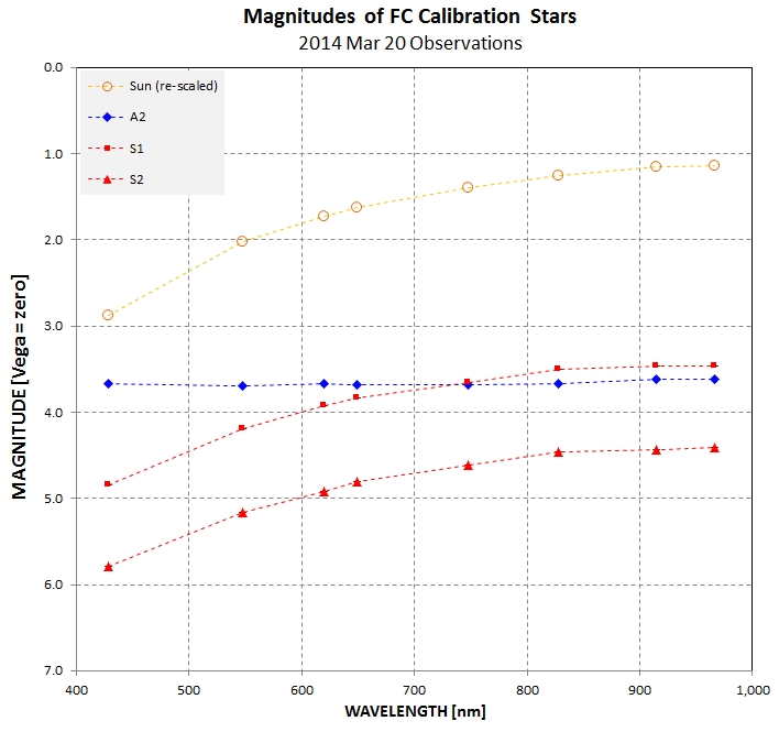
FC Secondary Calibration star magnitudes (Vega defined = zero).
As expected, star A2 is a flat line because it's the same spectral type as Vega. Also as expected, stars S1 and S2 have the same spectral "shape" as the sun because they're close to the same spectral type as the sun. Here's a table of FC Secondary Calibration star magnitudes.
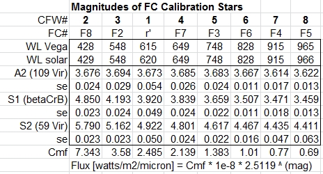
Table of FC Secondary Calibration star magnitudes. The equation for converting magnitude to flux is given.
Caption correction: Flux [watts/m2/um] = Cmf * 1e-8 * 2.5119 ^ (-mag).
2014.03.22. I'm still processing the Mar 20 image sets. All secondary stars that were observed on this date have been processed and provisional fluxes (& magnitudes) have been assigned to them. Below is a plot of their fluxes (on a log scale).
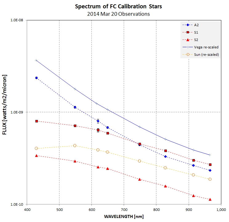
Flux spectrum of secondary standard stars A2 (109 Vir), S1 (beta CrB), S2 (59 Vir), compared with the re-scaled versions of Vega and solar spectra.
As expected, the A2 secondary star has a spectrum similar to Vega (since both have a spectral type of A0V). Als as expected, the two solar-like stars have a spectral shape similar to the sun's, although the shortest wavelength band doesn't have the same "drop" as the sun's spectrum (maybe related to lower metallicity).
An abundance of extinction slopes continue to support the earlier determination (this also supports the filter assignments to CFW location).
The only data from this observing date remaining to be processed are those for Vesta and Ceres.
2014.03.22. I'm still processing the Mar 20 image sets. The secondary standard star S2 has been calibrated.
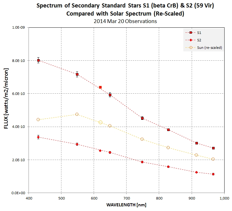
Flux spectrum of secondary standard stars S1 (beta CrB) & S2 (59 Vir), compared with the sun's spectrum (re-scaled).
Next up: calibration of secondary standard A2 (109 Vir). Then it will be Vesta and Ceres. When that's done the analysis for Mar 20 data will be complete.
2014.03.21. I'm still processing the Mar 20 image sets. The secondary standard star extinction curves look pretty good.
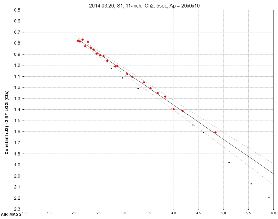
Extinction plot for secondary standard star S1 (beta Corona Borealis). Dot symbols represent data that exceed a chi-square acceptance threshold. The dotted traces are subjective stimates of a SE range.
The Vega extinction curves are noisier, due to 1) using 1-inch aperture, 2) short exposure times (0.3 to 10sec), and 3) observing at low elevations (13 - 30 deg). Some cirrus clouds were noted in my observing log for Vega observations, and they indeed are present at low level in the extinction plots. A method for identifying and disregarding the cirrus affected data has been developed, as the following two plots show.
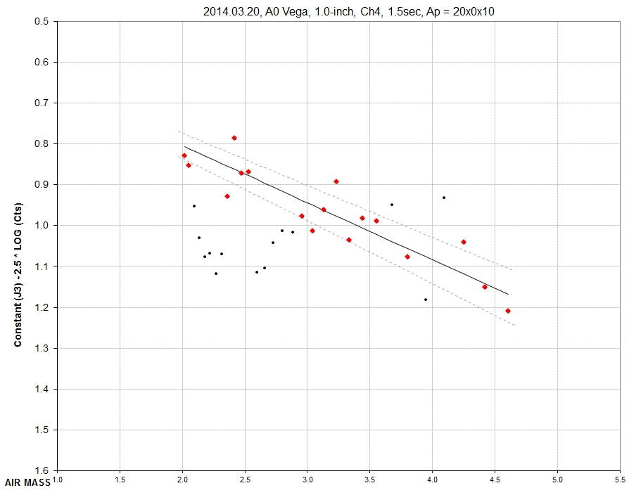
Vega extinction plot showing unaccepted data with small black dot symbols (caused by thin cirrus).
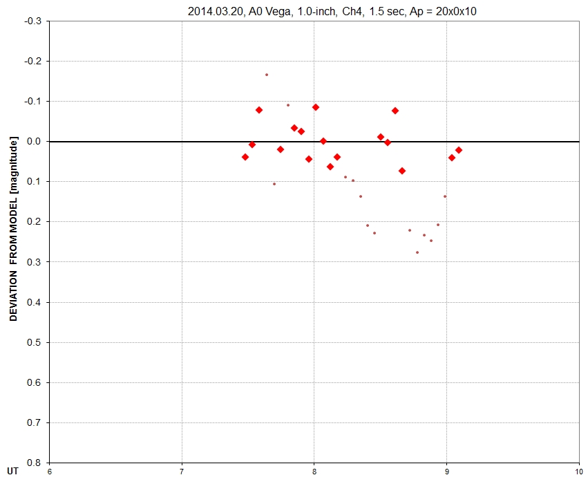
Departures from above extinction plot show when thin cirrus affected measurements.
Extinction spectra for S1 and Vega have been obtained, and they agree, as the following graph shows.
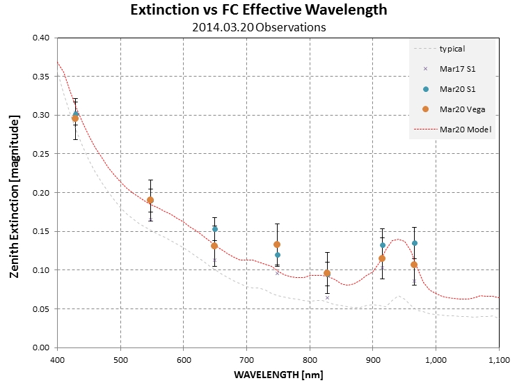
Extinction spectrum for Mar 20 data using stars Vega and S1. The model fit has 4 free parameters (Rayleigh scattering, stratospheric ozone, aerosol sccattering and water vapor burden), all of which have a priori uncertainties for the chi-square fitting.
The atmospheric extinction model is a strong guide in selecting an adopted set of extinction values for re-processing all data. For example, since star S1 provided better quality extinction estimates than Vega the final Vega fluxes are based on mostly S1 extinction solutions.
Secondary star S1 (beta Corona Borealis) has been calibrated to high accuracy from the Mar 20 data. It's spectrum resembles an "earlier" spectral type than I expected (based on B-V), as the following shows.
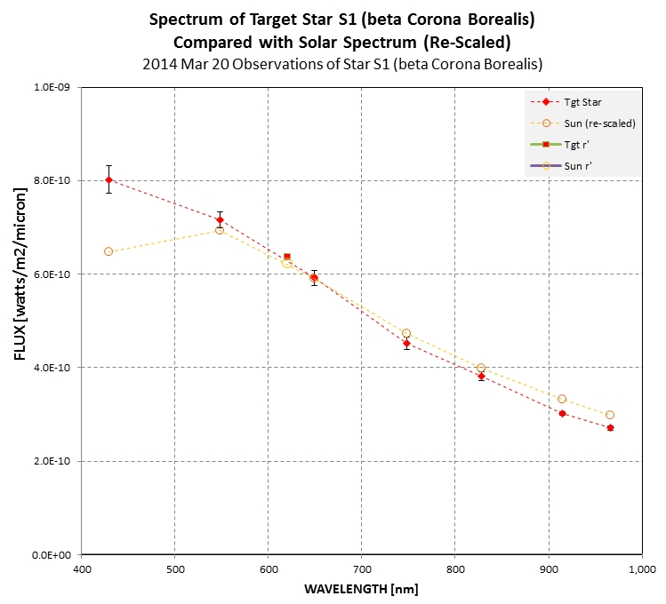
Flux spectrum of secondary standard S1 (beta CrB), compared with the sun's spectrum (re-scaled).
Error propagation is now included in the analysis.
Much analysis remains for the Mar 20 data set. Secondary standards S2 and A2, as well as Vesta and Ceres image sets, are ready for analysis using procedures developed for Vega and S1. The latest spreadsheet section for converting measured source counts (DN), apertures and exposure times to fluxes is shown below.
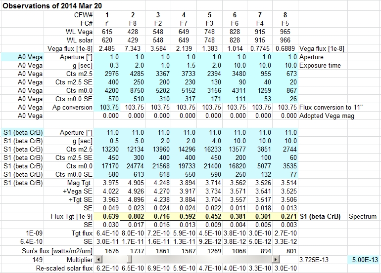
Example of spreadsheet section that converts measured source counts for a standard star (such as Vega) and a target star (such as S1) to fluxes at each FC band. Aqua colored cells are for user input (from another spreadsheet page) and the yellow cells are the "answer" (flux spectrum).
CFW#1 is a r'-band filter. The fluxes at r'-band will be used as a "sanity check" later because the literature has coefficients for converting r'-mag to flux. So far the r' fluxes agree with the flux spectrum based on FC filters, which is another sanity check.
2014.03.18. Refined non-parfocality focus offsets, and exposure times for A0V & solar type stars (to assure capability of sharp imaging when needed). Obs'd S1 (beta CrB), A2 (109 Vir) and S2 (59 Vir) for practice (there were cirrus clouds) in converting flux from an A-type star (the A stars in my list) to solar-type star (the S stars in my list). The image below is a screen capture of a spreadsheet showing how the A0V star "A2" (109 Virginis) was used to determine magnitudes for the sun-like star "S1" (beta Corona Borealis) at two bands. The star A2 was assumed to be exactly 3.730 magnitudes fainter than Vega in all bands (good assumption given that A2 has B-V ~ zero), and this permitted approximately correct assignment of the A2 star's flux for all bands. The zenith extrapolated magnitudes for A2 and S1 were entered into the spreadsheet and the fluxes for S1 were calculated (bottom row). Provision is made for entering which mask hole was used for each star (it was the 2.5" hole for both stars in this case). More than two bands weren't processed because this data is unsuitable for such an analysis due to the presence of cirrus clouds; this is just a demonstration of how magnitude systems can be created and used to convert to fluxes.
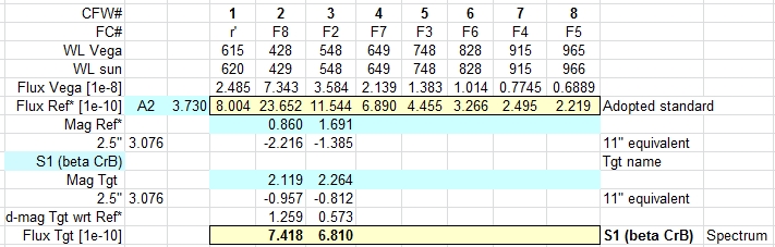
Demonstration of determining a solar-like star's spectrum by comparing its magnitude with an A-type star's magnitude for various filters. CFW# is "color filter wheel #." "WL Vega" is the Vega flux weighted wavelength for a band. "WL sun" is the solar spectrum weighted wavelength for a band. Flux values are in units [watts/m2/micron].
A Spectral Energy Distribution (SED) can be constructed from the data in the above spreadsheet. The SED version below is for Fλ [watts/m2/micron], and the sun's Fλ spectrum has been re-scaled for overlap to show shape similarity. A SED using λFλ using a log-log scale (commonly used) could also be easily created.
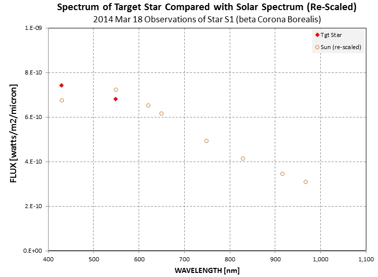
Example of spectrum of target star compared with the sun's spectrum (re-scaled).
2014.03.17. Obs'd sun-like star "59 Vir" (V=5.3) for 5 hours with all filters in order to establish a better quality extinction plot. There are two reasons for doing this: 1) to provide support to my proper identification of which filters are in the 10-position filter wheel locations (I was told they went from shortest WL to longest; only 3 had WL labels and at least they agreed with what I was told), and 2) to improve atmospheric extinction model for future use (I may need 2nd-order corrections for extinction when I'm transferring magnitudes from a secondary standard to a target, and if air mass values aren't exactly the same I'll need to perform small extinction corrections). The result is given below. This extinction plot is much better behaved than my first attempt, made the night before with a much more limited air mass range.
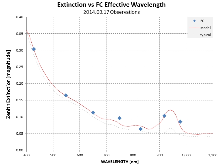
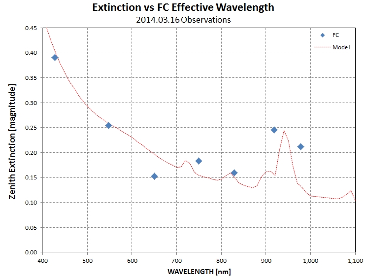
Measured zenith extinction vs. effective wavelength for FC filters for 2014.03.17. Model is a 40 nm wide smoothed version of a high resolution spectrum incorporating 1.3 x typical aerosol burden and 5 cm of precipitable water vapor (higher than expected for this season at my site).
Finalized list of A-type and solar-type stars for use as secondary standards.
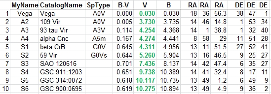
Calibration stars for this task. Vega is the primary standard (all mag's = zero), while the others are secondary standards.
2014.03.16. Obs'd 3 A-type stars and 3 G-type stars using all FC filters. Determined extinction for all bands (graph below), and they are compatible with a model atmosphere. The model includes 6 cm precipitable water vapor (higher than I think is likely) and 3 times greater than typical aerosol burden (quite possible given that the previous day was hazy due to wind-blown dust). Determined magnitude differences observing through an aperture mask with 1.0- and 2.5-inch holes that can be flipped open or closed for accommodating very bright stars (such as Vega): 11-inch to 2.5-inch produces 3.076 ± 0.010 magnitude difference, 11-inch to 1.0-inch produces 5.040 ± 0.010 magnitude difference. A star with same B-V as Vega was included among the A-type stars observed; it has B and V magnitudes of ~3.732, so by adjusting its flux by the factor 2.512-3.732 = 0.0321 it should be possible to obtain an approximate calibration of the 3 sun-like stars (magnitudes on a scale with Vega as zero for all bands), which would then allow any magnitudes based on these sun-like stars to be converted to flux [watts/m2/micron].