TRANSMISSION GRATING SA-100 AND CERES SPECTRUM
B. Gary, Last modified 2015.07.31
This web page describes how I have used the
SA-100 transmission grating to create a spectrum of Ceres
for ~ half of a rotation. I conclude that I don't know how
to obtain and process SA-100 images for achieving spectra
that are as accurate as can be obtained using the FC
filters. This conclusion is based on the finding that the
variation of geometric albedo with rotation is slightly
greater for the SA-100 data than the FC data.
Observations
After several short observing sessions devoted to learning how to
observe with the SA-100, and reduce the images, I observed Ceres on
two nights: Jun 05 (cut short by clouds) and Jun 06 (lasting 4.5
hrs, from twilight to Ceres setting below20 degrees). A sun-like
secondary standard star (59 Vir) was observed at intervals of ~1 hr
for ~ 15 min. Exposure times were 4 seconds for 59 Vir and 10
seconds for Ceres, which assured that the spectrum would not be
saturated. On May 31 Gamma UMa was observed for the purpose of
establishing pixel to wavelength conversion equation.
Reduction Process
Standard calibrations were used for all images (bias, dark and
flat). Groups of images for a target (GUMa, 59 Vir or Ceres) were
aligned, checked for quality (sharpness & lack of cloud effects)
and median combined. The combined images was then measured using a
horizontal box photometry tool in MaxIm DL (Fig. 1).
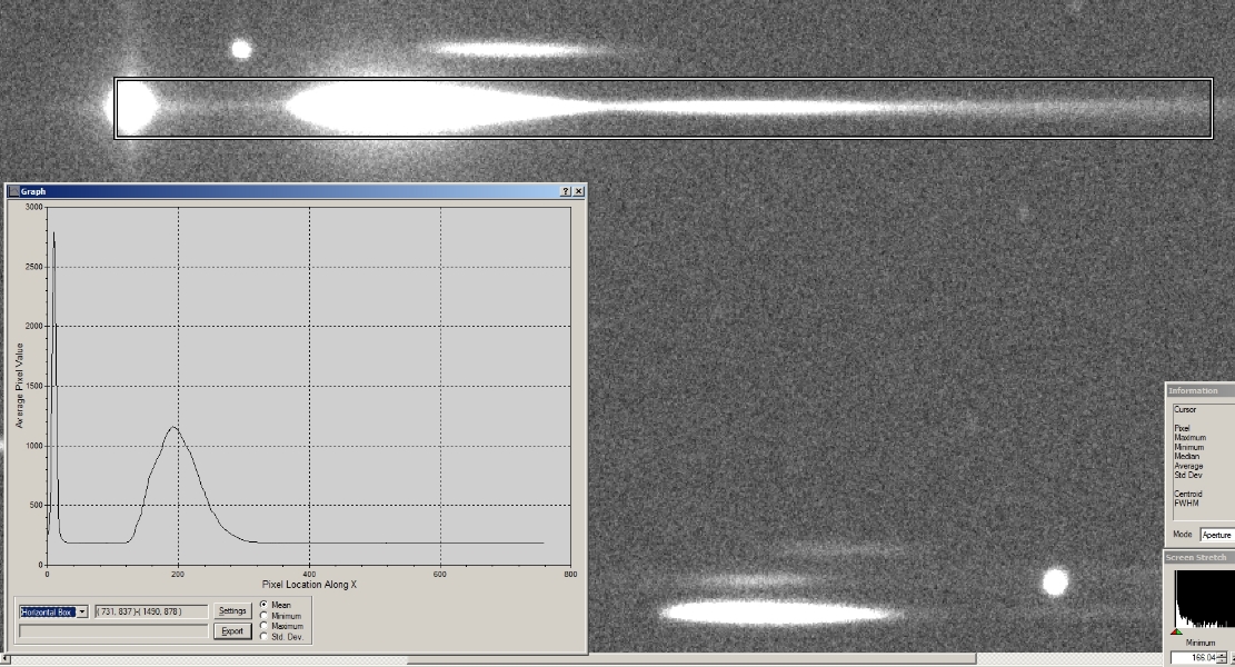
Figure 1. Horizontal box photometry of spectrum,
extending from zeroth-order star-like image through the 1st-order
spectrum and including most of the 2nd-order spectrum.
The csv-file produced from the box photometry tool is imported to a
spreadsheet which I have designed for analysis of the SA-100 data. A
baseline is created that can be adjusted by the user for offset,
slope and 2-nd-order pixel offset, height and width (Fig. 2). The
2nd-order baseline component is a re-scaled version of the 1st-order
spectrum, which is adjusted for intensity rescaling, pixel location
offset and width (typically 1.47 times wider).
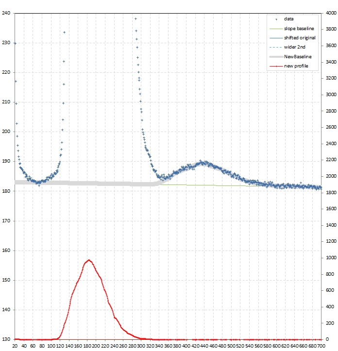
Figure 2. Baseline (thick gray trace) adjusted by user for
intensity offset and slope. A version of the 1st-order spectrum is
shifted to a 2nd-order pixel location; it is re-scaled and
also widened by a factor ~ 1.48. The red trace at
the bottom is what is left after subtracting the user-adjusted
baseline.
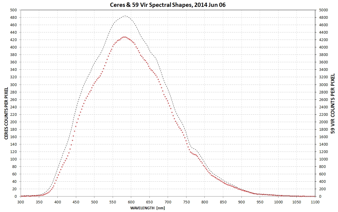
Figure 3. An observed spectrum of Ceres and
standard star 59 Vir. Note the telluric oxygen absorption
feature at 763 nm, and the very low intensity beyond ~1000 nm.
This figure illustrates the importance of carefully establishing a
baseline for both the standard star and Ceres. It also can be used
to visualize the errors that can occur if either has an incorrectly
shifted wavelength adjustment (which is done manually for each
spectrum, as described below).
Calibration of the pixel value to wavelength is accomplished using a
star with many known absorption lines. Gamma Ursa Majoris (GUMa) is
a A0V star which is ideal for this purpose (Fig. 4).
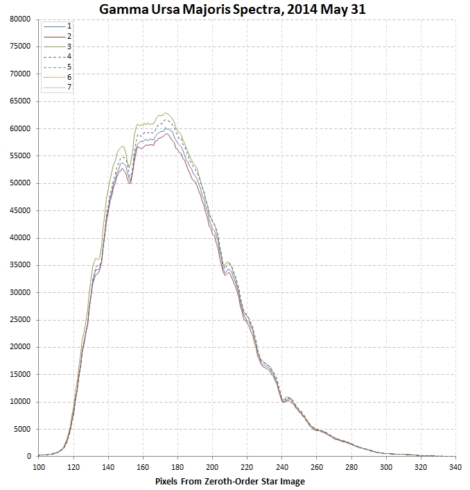
Figure 4. Four spectra of Gamma Ursa Majoris, showing
several Balmer lines and some telluric (atmospheric) absorption
features.
To see the absorption lines better I have created a "spectral
structure" plot, using "intensity / smoothed intensity" (Fig. 5).
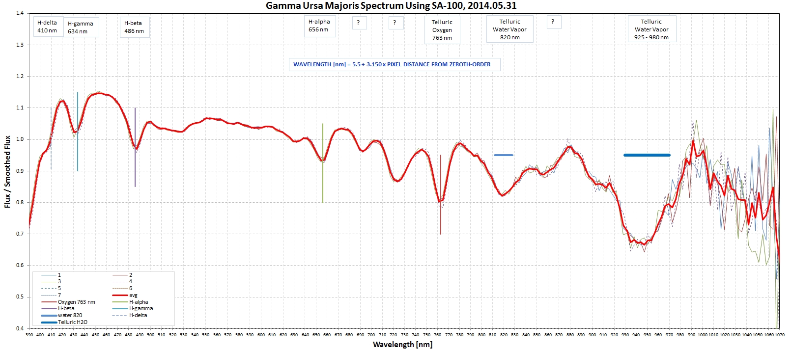
Figure 5. Gamma UMa "spectral structure" (intensity /
smoothed intensity) used to establish the pixel to wavelength
conversion equation.
Provided image scale doesn't change the equation for converting
"pixels from zeroth-order location" to wavelength should be the same
throughout an observing session, and from night-to-night. However, I
found it convenient to use the telluric oxygen absorption feature at
763 nm for providing a final wavelength shift adjustment. Since this
absorption feature is produced by the atmosphere it is present in
every spectrum. Notice that the complex of water vapor absorption
lines in the 930 to 990 nm region can mimic the 1 micron pyroxene
Band I with a minimum at between 920 and 945 nm.
For an observing session I process all the 59 Vir (sun-like
secondary standard star) images to produce a set of spectra with a
spacing of ~ one hour. The first and last observations are always of
this star, which assures that any changes in atmospheric extinction
can be modeled for use with Ceres. The atmospheric extinction model
has a resolution of one pixel's worth of wavelength (3.2 nm), and it
consists of two components: an overall extinction for the night and
a table of departures versus UT. I don't determine all of these
parameters for each 3.2 nm interval; rather, I create "pseudo filter
bands" by averaging over the FC bandpasses, and for each of these
bands I plot log(Intensity) vs. air mass and "departure vs UT"
(where "departure" is a visual reading of plotted difference from
the air mass fit at 3 UT times), as shown in Fig. 6.
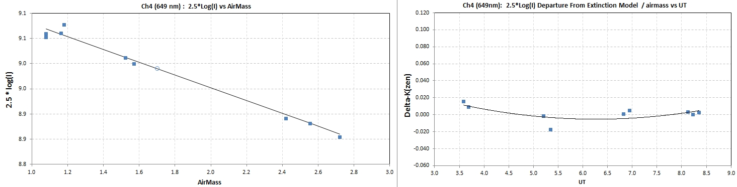 Figure 6. Calibration star (59 Vir)
"pseudo FC band #6" log(Intensity) vs air mass with a
simple atmospheric extinction fit (left) and plot of departures of
panel a data vs. UT.
Figure 6. Calibration star (59 Vir)
"pseudo FC band #6" log(Intensity) vs air mass with a
simple atmospheric extinction fit (left) and plot of departures of
panel a data vs. UT.
In the above figure the slope of 2.5*Log(Intensity) vs. air mass was
fit using an atmospheric model constrained to have physically
reasonable values for Rayleigh scattering, ozone absorption, aerosol
scattering and water vapor absorption. The user can adjust a
multiplier for each of these for extinction components subject to
the a priori constraints. A Bayesian procedure could have
been used but was not considered necessary at this early stage in
assessing the SA-100.
After completing the calibration star reduction the Ceres image sets
are grouped and median combined, etc, similar in manner to the
procedure used for the calibration star. Groups of ~30 stars are
typically "loaded" into MaxIm DL for review, and a PSF FWHM
criterion is chosen for deleting images with poor "seeing" or
tracking. Typically, 1/2 to 2/3 of the group is accepted for median
combining (after Ceres "star alignment"). The horizontal box
photometry file is imported to the spreadsheet, and baseline
subtraction is performed in the same manner as for the calibration
star - whose results reside in a special place for comparison with
Ceres. After each median combined image photometry is processed the
baseline subtracted counts spectrum is copied to a spreadsheet page
for additional processing. The Ceres counts spectrum is divided by a
version of the calibration star counts spectrum that the extinction
model predicts would have been observed at the Ceres air mass and
UT. This ratio is multiplied by the ratio "sun's flux / calibration
star flux" versus wavelength. The result of this is a "Ceres flux /
sun's flux" spectrum, which can be converted to geometric albedo
using the standard parameters (r, d R, G). I've chosen the G vs
wavelength result that I obtained using FC filters (fitted with a
polynomial), shown as Fig 7.
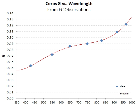
Figure 7. Phase effect parameter G versus wavelength based
on FC filters for April and May, 2014.
Each image group leads to a spectrum, as shown in Fig. 8.
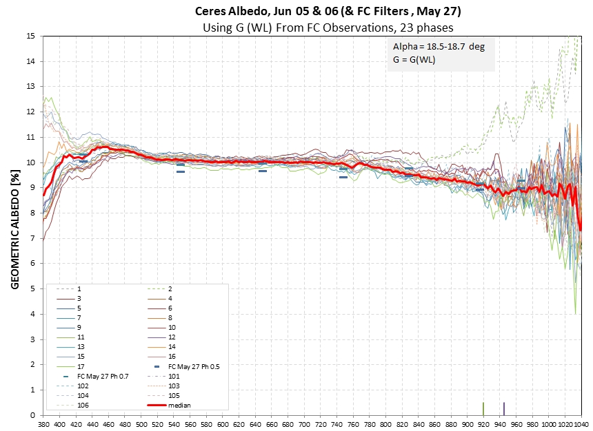
Figure 8. Spectra for 23 image groups, with rotation
phases ranging from 0.13 to 0.64 (using an ephemeris where
rotation phase is zero at JD = 2456736.73). Note the pairs of
horizontal symbols at the FC wavelengths, which are measure
geometric albedo for May 27.
Several results can be taken from this figure. First, the overall
geometric albedo using the SA-100 is the same as for the FC filters.
This is gratifying because completely different observing and
reduction procedures are used for the two methods. This is the only
positive result. The rest are negative!
At the short and long ends of the spectrum there are wild variations
of albedo. At the long end two problems exist: 1) the spectra are
noisy, and 2) there is a systematic problem with two traces. These
two traces were made when a nearby star was producing a spectrum
that overlay the Ceres spectrum. Refer back to Fig. 1 to see this
star, which was moving with respect to Ceres in a manner that placed
them at the same declination when the two outlier Ceres spectra were
obtained. I note that a slit spectrograph would not have this
problem. The noisiness is cased by the instrumental response
function going to zero at ~ 1100 nm, caused by corrector plate
transmission, focal reducer lens transmission, SA grating
transmission and CCD QE.
At the short wavelength end of the spectrum there is also a problem
with instrumental response function, but the sun's spectrum also
falls off fast with wavelength in this region. I think baseline
fittings are difficult here because the zeroth-order PSF overlaps
the short wavelength end of the 1st-order spectral region (refer to
Fig. 2 to see this). The wild variations at wavelengths below ~ 460
nm may be caused by 1) weak solar flux combined with an uncertain
baseline fitting, 2) steep decline of solar flux with decreasing
wavelength combined with errors in aligning Ceres spectra with the
average 59 Vir standard star spectrum.
The spectral region 460 to 680 nm is "well-behaved," and from 680 nm
to ~ 920 nm most spectra agree with each other. The geometric albedo
at 548 nm, for example (an FC band), has internal consistency that
can be accounted for if each value has SE = 0.07 (based on neighbor
differences). To use a specific example, at phase 0.478 the 548 nm
SA-based geometric albedo = 10.01 ± 0.07 %, where the stated SE is
the stochastic component. The systematic component of uncertainty is
more difficult to estimate. This is comparable to the FC-based
geometric albedo stochastic component; so for this band it should be
possible to construct a phase-folded geometric albedo light curve,
as in Fig. 9, below.
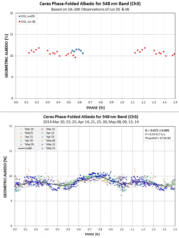
Figure 9. Phase-folded geometric albedo based on SA-100
observations (top) and FC filters (bottom).
The SA-100 phase-folded geometric albedo plot is compatible with the
corresponding plot based on FC filters provided allowance is allowed
for a G adjustment (since SA gives 10.15% vs FC's 9.75%). There is
insufficient data to verify similarity of structure with rotation.
The one unique value in the SA-100 observations of Ceres, over the
FC counterparts, is more spatial resolution. Referring to Fig. 10,
below, the Band I feature is present, and possibly useful for
assessing mineralogy. However, the data in this region is so
noisy that this use for the SA100 data is questionable.
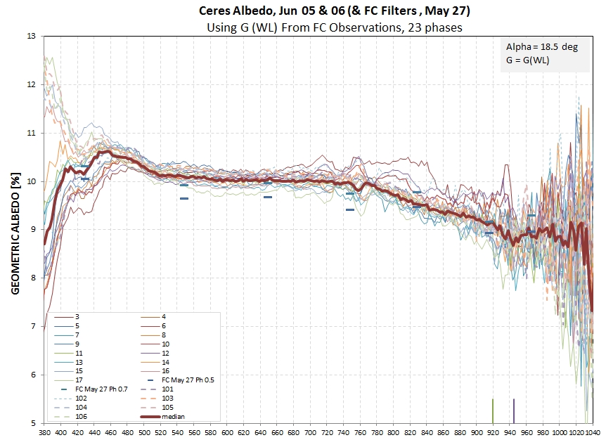
Figure 10. Plot of "median" spectrum of each
geometric albedo plot for Jun 05 & 06, showing an un-useable "Band
I" feature with a minimum at ~ 940 nm.
A small "Band I" feature is present, but the noisiness of even the
median spectrum renders it essentially useless. Data quality in this
region is affected by the water vapor absorption feature at the same
wavelength region.
SA-100 Limitations
Consider the spectrum of Ceres as observed after instrumental losses
caused by the atmosphere, corrector plate transmission, focal
reducer transmission, SA-100 grating transmission and CCD QE.
Repeat of Figure 3. An observed spectrum of Ceres and
standard star 59 Vir. Note the telluric oxygen absorption
feature at 763 nm, and the very low intensity beyond ~1000 nm.
At the long wavelength end measured flux is so low that small
changes in baseline fitting, for either Ceres or the standard star,
can produce large changes in flux ratio. At the short wavelength end
small changes in adopted wavelength shift (using the 763 nm telluric
absorption feature) can produce large changes in flux ratio. It's my
assessment that these two factors are the principal explanations for
the large variations in geometric albedo (exhibited in Fig.'s 8 and
10). Another problem with using the SA-100 is something all
transmission gratings must deal with: because transmission gratings
don't use a slit the spectrum is superimposed upon a background of
stars, as well as the spectra of those stars. Even when this problem
is not obvious, as happened to cause the two outlier spectra in Fig.
8, these problems are present at lower levels for most other
spectra. Their effect will of course be more noticeable for regions
where the Ceres spectrum is faint, which may be a significant
contributor for the noisiness at the short and long wavelength ends
of the spectrum.
Some of these problems could be alleviated by improving the
instrumental response function. My Meade telescope's Cassegrain
corrector plate, and the focal reducer, contribute to reduced
response at the wavelength extremes. These components would not be
present in a reflective optics only configuration. My ST-10XME CCD's
QE is "enhanced" at the blue end, but the red end QE response
fall-off is due to fundamental properties of silicon physics.
Instrumental system response can be estimated from the ratio of a
star's measured counts spectrum to it's actual flux spectrum, with
an adjustment that produces a value at mid-wavelengths that can be
calculated from documented performance specifications. This is
shown in the next figure.
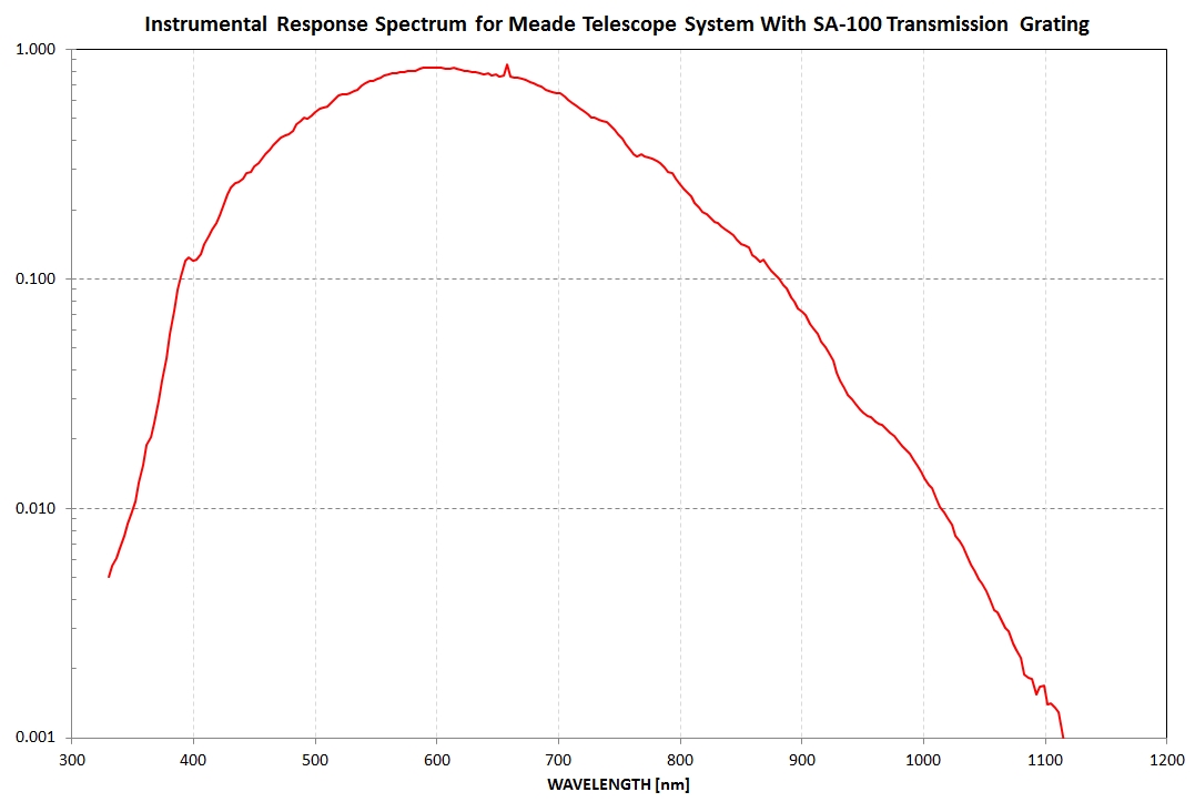
Figure 11. Estimated "instrument system response
function" for my Meade telescope, with focal reducer, SA-100 and
ST-10XME CCD. (The feature at 763 nm is due to the way this trace
was produced: ratio of measured spectrum to known flux spectrum,
adjusted at ~ 600 nm to be ~ 0.90).
The "instrumental response function" is > 50% from 480 nm to 780
nm, and the geometric albedo results are "well behaved" in that
region. Clearly, one way to improve results with the SA-100 is to
improve instrumental response by reducing transmission losses at the
short and long wavelengths (i.e., using a reflective-only telescope
system).
All-sky photometry with filters is less affected by a falling-off
response function. This is due to several factors, but one is the
fact that the spectral response function is not subject to user
adjustments (meant to overcome changes in image scale as well as not
knowing the exact location of the zero-order image due to PSF
distortions and saturation). Another factor favoring filters where
the response function is low is not having to rely upon user
adjustments of a spectrum baseline. Finally, a filter system is not
affected by order-overlap, which requires subjective modeling for
the transmission grating observations.
Based on observations of asteroid BL86 (V = 9.5) and 2011 UW158 (V =
15.5) I can estimate the region in wavelength/magnitude space where
SA1-00 observations are feasible with a 14" telsecope.
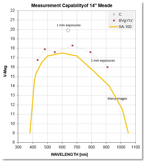
Figure 12. Measurement capability region for 14"
telescope with SA-100 (yellow trace), assuming use of star
subtraction, asteroid alignment and median combining of many
images. For comparison, limiting magnitudes are shown for Clear
and BVg'r'i'z' filters (60 second exposures, SNR = 3, 2.3
"arc FWHM).
To illustrate use of this figure, it is possible to observe the
spectrum of an asteroid from 400 to 950 nm when it is at V-mag =
13.0.
In Conclusion
After taking my time trying to do the best possible job of
processing SA-100 images of Ceres and a nearby calibration star, and
because of the additional precautions I've incorporated for the
SA-100 reduction I now can state that the SA-100 reduction process
is more work than the FC reduction process. I think the SA-100
geometric albedo quality is slightly inferior to the FC albedo
quality at the shortest and longest wavelengths, and I propose
discontinuing observations with the SA-100 and returning to use of
the FC filters.
Links
Star Analyzer
home page
Master
list of B. Gary web sites
________________________________________________________________
This site opened: 2014.06.08. Webmaster: Bruce L. Gary