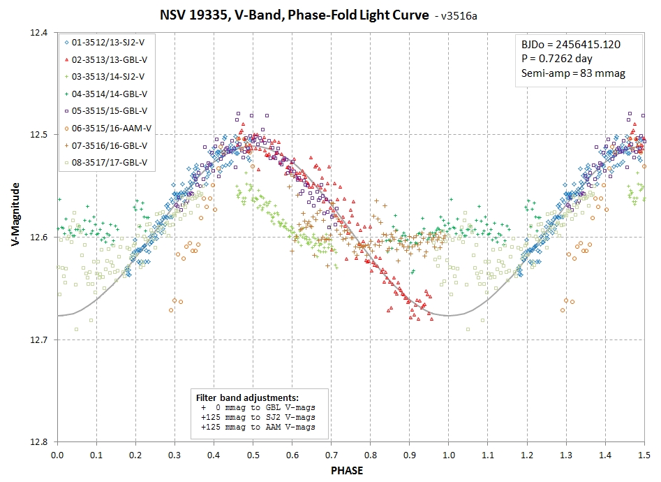
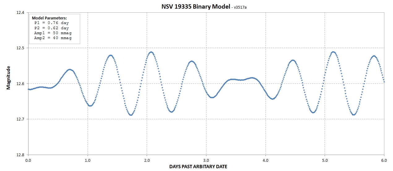
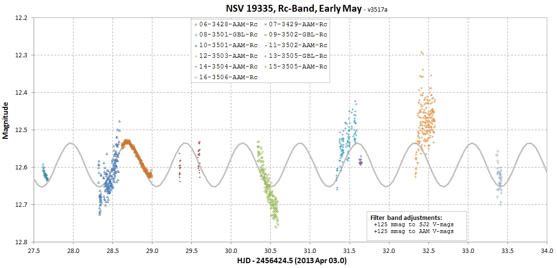
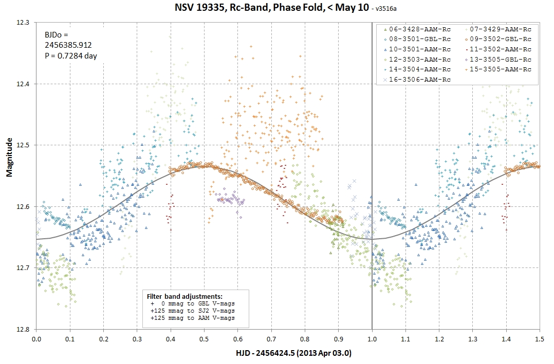
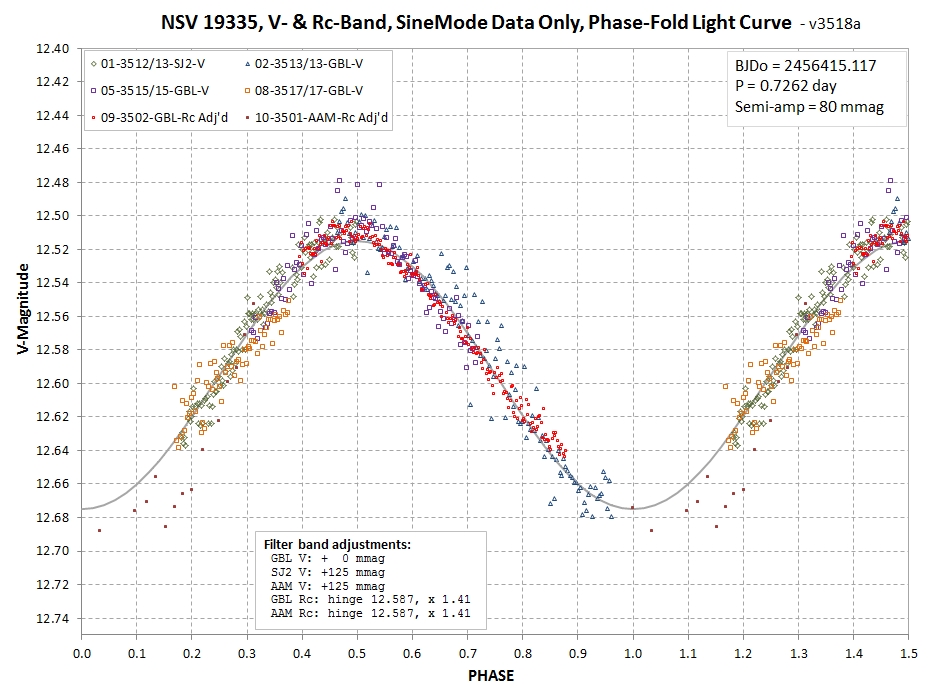
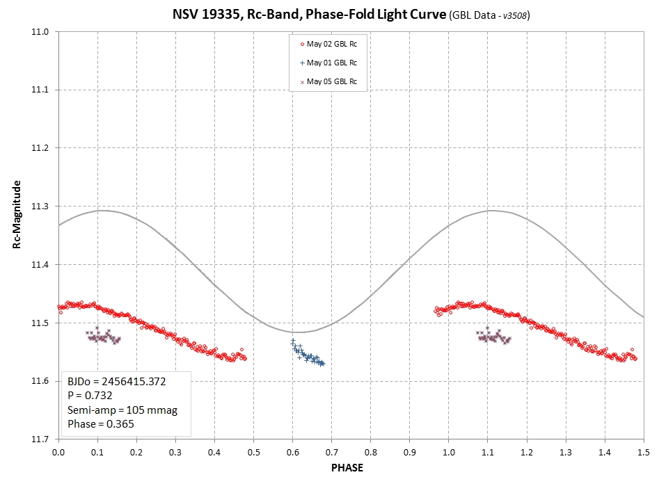
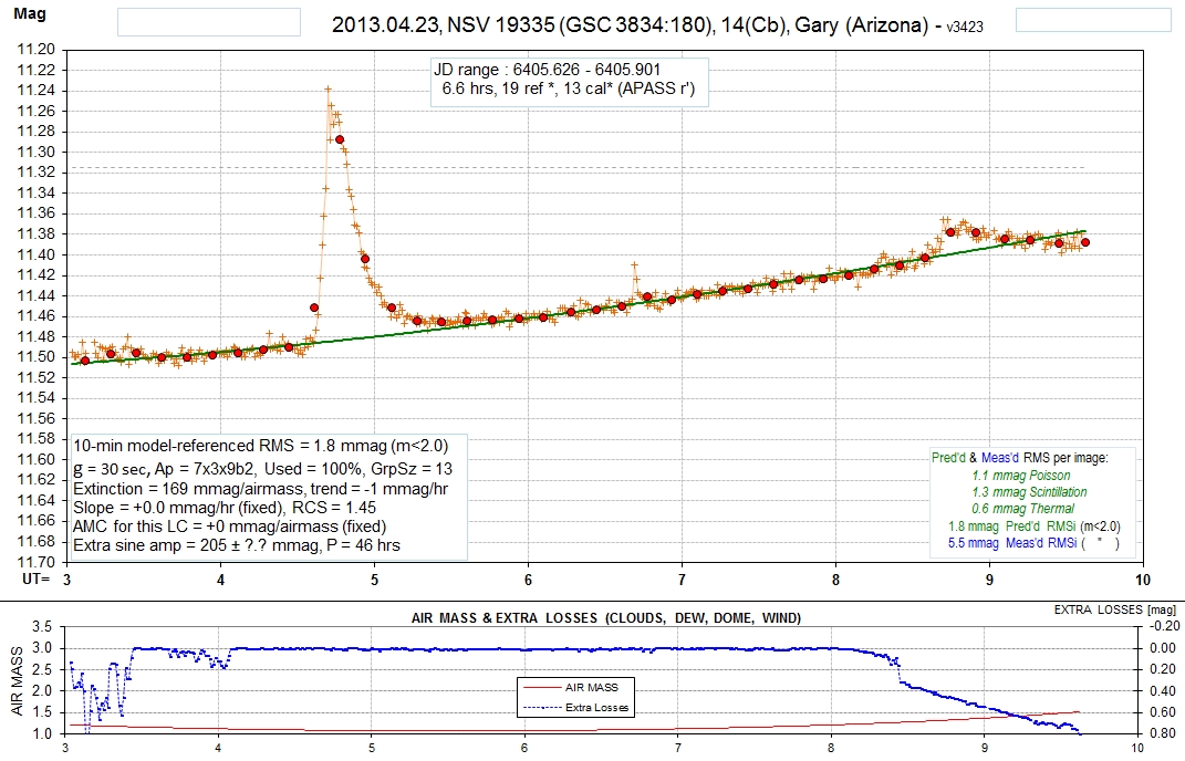
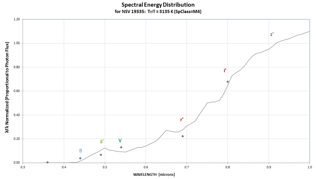
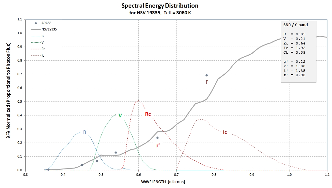
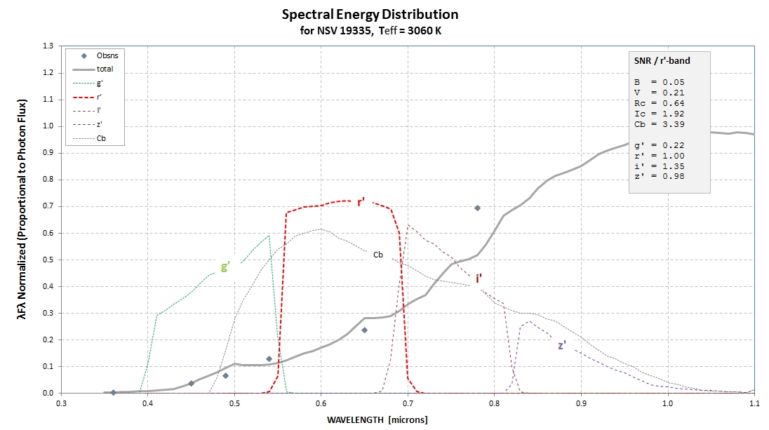
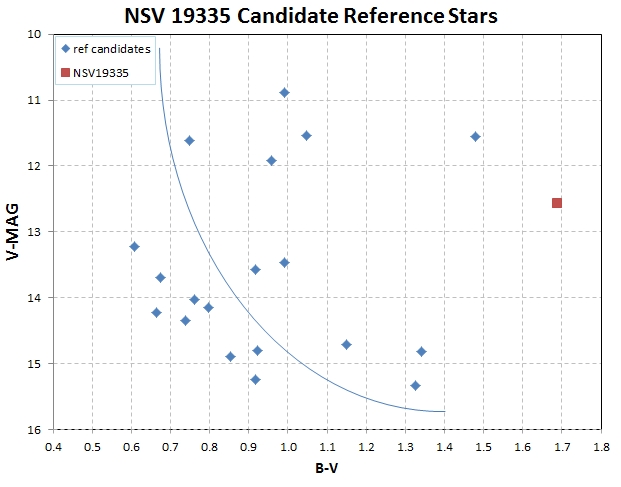
This web page describes a project of coordinated observations of an M dwarf star that has puzzling variations in multi-band observations. Observations by a team of European and American amateurs is underway. Observing dates and filter use is being coordinated in a way that will address the reality of departures from a single sinusoidal variation. It is anticipated that observations will be confined to 2013 May and June.
| Session #1 |
Session #2 |
Session #3 |
Session #4 |
Session #5 |
Session #5.5 |
Session #6 |
Session #7 |
Session #8 |
Session #9 |
|
| Sunday May 12/13 |
Monday May 13/14 |
Wednesday May 15/16 |
Thursday May 16/17 |
Saturday May 18/19 |
Sunday
May 19/20
|
Monday May 20/21 |
Wednesday May 22/23 |
Friday May 24 |
||
| Ogmen |
cloudy | cloudy | Rc, 18.0-22.2 on
18th |
Rc, 20.0-22.0 |
||||||
| Arminski |
rain |
rain |
V, 21.5-26.3, 15th |
cloudy | OVC |
V, 21.8-25.3 |
||||
| Zambelli |
cloudy | cloudy | cloudy | cloudy | OVC |
vacation |
||||
| Salas |
V, 21.9-27.5, 12th |
V, 20.2-25.0 |
cloudy | cloudy | raining |
OCV |
||||
| Gregorio |
down for repair |
down for repair | V, 2.9-9.9, 16th |
cloudy | BKN, not obs'g |
BKN |
Rc,
obs'g |
|||
| Gary |
V, 02.8-11.5, 13th |
V, 02.8-9.8, 14th |
V, 2.8-9.9, 16th |
V,
2.8-10.0, 17th |
Rc, 4.2-11.2 on19th |
r',
03.0-11.3 |
r', 3.3-10.2 |
|||
| Wiggins |
cloudy |
cloudy |
cloudy | cloudy | cloudy |
Rc, 4.3-10.1 |
Rc,
4.5-10.1 |
|||
| Foote J |
on travel |
on travel | cloudy | cloudy | cloudy |
on travel |
||||
| Foote C |
on travel |
on travel | cloudy | cloudy | cloudy |
on travel |
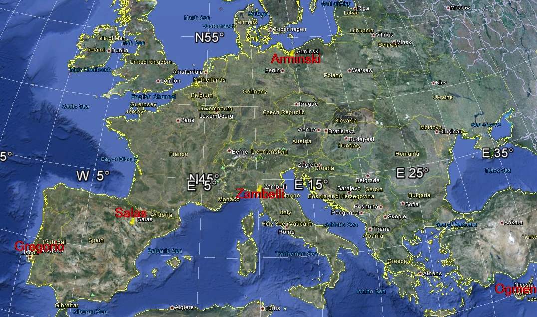
| East Longitude (Lat) |
Observer Name (Code) |
Location |
Telescope & Filters | E-mail |
|
| +033.725 (+35.258) |
Yenal Ogmen (OYE) |
North Cyprus |
14": B, V, Rc,Ic |
green.island.observatory at live.com |
more
info |
| +014.550 (+53.4??) |
Andrzej Arminski (AAM) |
Szczecin, Poland |
08": V, Rc |
aa at aarminski.com.pl |
more
info |
| +010.008 (+44.104) |
Roberto Zambelli (ZRO) |
Sarzana, Italy |
16": V, LRGB |
robertozambelli .rz at libero.it |
more
info |
| -000.936 (+41.629) |
Javier Salas (SJ2) |
Saragossa, Spain |
14": B, V, R, I, Cb |
jsalas at orange.es |
more
info |
| -008.817 (+38.733) |
Joao Gregorio (GJL) |
Atalaia, Portugal |
12": V,Rc,Ic,L,Cb |
crisostomo.gregorio at oninet.pt |
more
info |
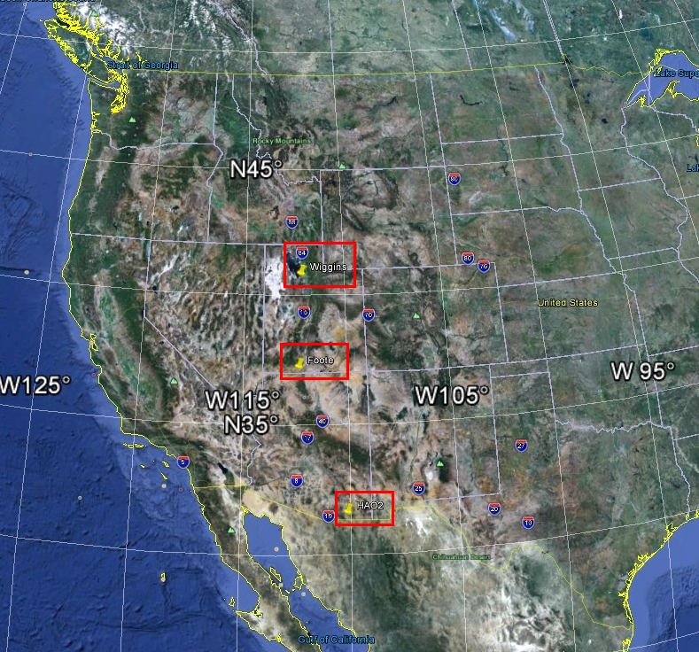
| -110.238 (+31.452) |
Bruce Gary (GBL) |
Hereford, Arizona; USA |
11": B, V, Rc, Ic, Cb, g', r', i', z' |
brucegary9 at gmail.com |
more
info |
| -112.296 (+40.641) |
Patrick Wiggins (WPK) |
Stansbury Park, Utah; USA |
14": B, V, R, I, C (Schuler) |
paw at wirelessbeehive.com |
more
info |
| -112.435 (+37.029) |
Jerry Foote (JFEA) |
Kanab, Utah; USA |
24": B, V, Rc, Ic, C |
jfoote at kanab.net |
more
info |
| -112.436 (+37.028) | Cindy Foote (FCN) |
Kanab, Utah; USA |
16": V, V, Rc, Ic, C |
cfoote at kanab.net |
more
info |
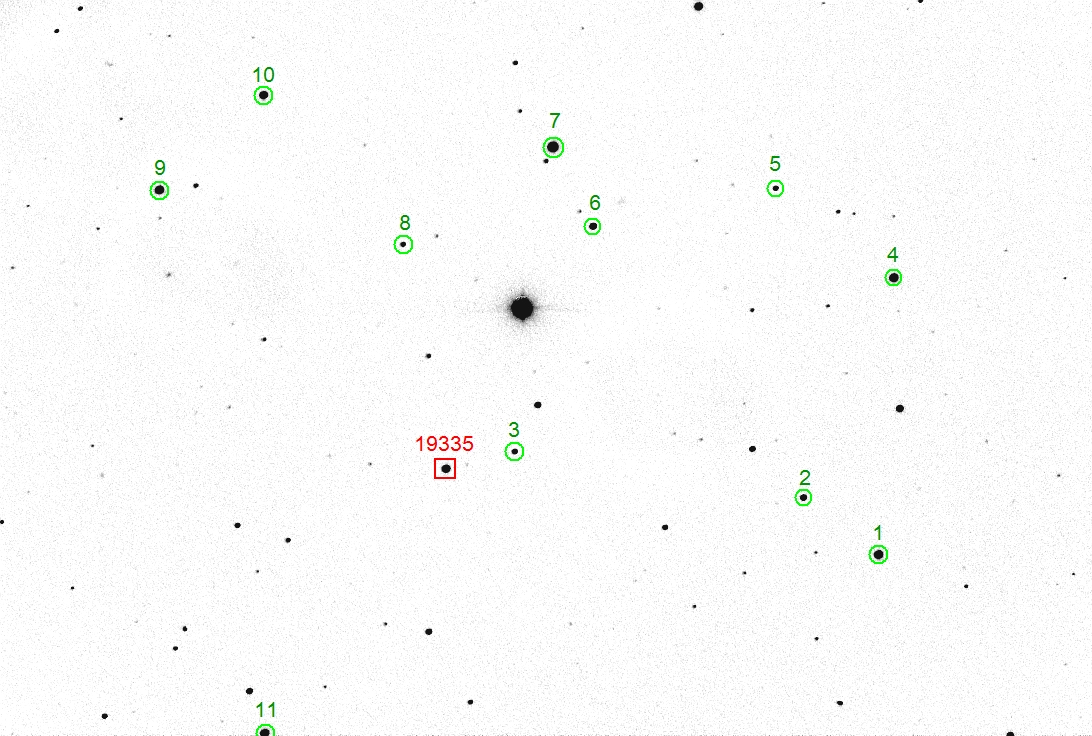
| Ref# |
B |
V |
Rc |
Ic |
g' |
r' |
i' |
z' |
B-V |
| 1 |
13.033 |
11.554 |
10.385 |
10.775 |
12.291 |
11.084 |
10.634 |
10.385 |
1.479 |
| 2 |
14.487 |
13.571 |
13.065 |
12.650 |
14.004 |
13.303 |
13.098 |
13.027 |
0.916 |
| 3 |
16.156 |
14.816 |
13.987 |
13.414 |
15.523 |
14.298 |
13.935 |
13.787 |
1.340 |
| 4 |
12.593 |
11.546 |
11.007 |
10.528 |
12.043 |
11.257 |
10.988 |
10.850 |
1.047 |
| 5 |
15.865 |
14.716 |
14.027 |
13.480 |
15.320 |
14.309 |
13.972 |
13.829 |
1.149 |
| 6 |
14.452 |
13.460 |
12.939 |
12.501 |
13.927 |
13.183 |
12.955 |
12.868 |
0.992 |
| 7 |
11.876 |
10.884 |
10.373 |
9.891 |
11.344 |
10.615 |
10.343 |
10.192 |
0.992 |
| 8 |
16.662 |
15.337 |
14.490 |
13.877 |
16.029 |
14.802 |
14.399 |
14.226 |
1.325 |
| 9 |
12.869 |
11.912 |
11.421 |
10.929 |
12.361 |
11.659 |
11.377 |
11.227 |
0.957 |
| 10 |
13.178 |
12.410 |
12.012 |
11.643 |
12.745 |
12.225 |
12.066 |
12.008 |
0.768 |
| 11 |
12.355 | 11.607 | 11.232 | 10.864 | 11.956 |
11.444 |
11.286 |
11.220 |
0.748 |

| Ref# |
B |
V |
Rc |
Ic |
g' |
r' |
i' |
z' |
B-V |
| 1 |
13.033 |
11.554 |
10.385 |
10.775 |
12.291 |
11.084 |
10.634 |
10.385 |
1.479 |
| 2 |
14.487 |
13.571 |
13.065 |
12.650 |
14.004 |
13.303 |
13.098 |
13.027 |
0.916 |
| 3 |
16.156 |
14.816 |
13.987 |
13.414 |
15.523 |
14.298 |
13.935 |
13.787 |
1.340 |
| 4 |
12.593 |
11.546 |
11.007 |
10.528 |
12.043 |
11.257 |
10.988 |
10.850 |
1.047 |
| 5 |
15.865 |
14.716 |
14.027 |
13.480 |
15.320 |
14.309 |
13.972 |
13.829 |
1.149 |
| 6 |
14.452 |
13.460 |
12.939 |
12.501 |
13.927 |
13.183 |
12.955 |
12.868 |
0.992 |
| 7 |
11.876 |
10.884 |
10.373 |
9.891 |
11.344 |
10.615 |
10.343 |
10.192 |
0.992 |
| 8 |
16.662 |
15.337 |
14.490 |
13.877 |
16.029 |
14.802 |
14.399 |
14.226 |
1.325 |
| 9 |
12.869 |
11.912 |
11.421 |
10.929 |
12.361 |
11.659 |
11.377 |
11.227 |
0.957 |
| 10 |
13.178 |
12.410 |
12.012 |
11.643 |
12.745 |
12.225 |
12.066 |
12.008 |
0.768 |
| 11 |
13.837 | 13.230 | 11.232 | 10.864 | 13.537 |
12.982 |
12.009 |
11.220 |
0.607 |
| East Longitude (Lat) |
Observer Name (Code) |
Location |
Telescope & FiltersData sub | E-mail |
|
| +033.725 (+35.258) | Yenal Ogmen (OYE) |
North Cyprus | 14": B, V, Rc,Ic | green.island.observatory at live.com | more info |
| +014.550 (+53.4??) |
Andrzej Arminski (AAM) |
Szczecin, Poland |
08": V, Rc |
aa at aarminski.com.pl |
more
info |
| +010.008 (+44.104) |
Roberto Zambelli (ZRO) |
Sarzana, Italy |
16": V, LRGB |
robertozambelli .rz at libero.it |
more
info |
| -000.936 (+41.629) |
Javier Salas (SJ2) |
Saragossa, Spain |
14": B, V, R, I, Cb |
jsalas at orange.es |
more
info |
| -008.817 (+38.733) |
Joao Gregorio (GJL) |
Atalaia, Portugal |
12": V,Rc,Ic,L,Cb |
crisostomo.gregorio at oninet.pt |
more
info |
| -110.238 (+31.452) |
Bruce Gary (GBL) |
Hereford, Arizona; USA |
14": B, V, Rc, Ic, Cb, g', r', i', z' |
19335 at brucegary.net |
more
info |
| -112.296 (+40.641) |
Patrick Wiggins (WPK) |
Stansbury Park, Utah; USA |
14": B, V, R, I, C (Schuler) |
paw at wirelessbeehive.com |
more
info |
| -112.435 (+37.029) |
Jerry Foote (JFEA) |
Kanab, Utah; USA |
24": B, V, Rc, Ic, C |
jfoote at kanab.net |
more
info |
| -112.436 (+37.028) | Cindy Foote (FCN) |
Kanab, Utah; USA |
16": V, V, Rc, Ic, C |
cfoote at kanab.net |
more
info |