Occasionally I notice that a new observer is using procedures for observing and image analysis that are meant for use with variable star tasks and which therefore are not optimized for the task of exoplanet observing. Whereas experience with AAVSO tasks is helpful to someone starting to observe exoplanets, the two tasks are different enough that many of the procedures for AAVSO tasks should not be adhered to while learning to observe exoplanets. This web page is meant to highlight the differences, and provide ideas for adjusting strategies in observing, image measurement and spreadsheet analysis that will benefit the results for exoplanets.
INTRODUCTION TO HOW EXOPLANET AND AAVSO VARIABLE STAR OBSERVING AND ANALYSIS DIFFER
Most AAVSO tasks have the goal of monitoring changes in a star's brightness from one night to another. This requires the use of nearby reference stars, that are still referred to by the term "comparison stars" (revealing that the term originated in the days when visual observing was employed). Each reference star must have a known brightness for each filter band, and these brightness values must be the same for time scales of years and decades. Since variations of the target star's brightness will be inferred by comparing measurements by different observers it is necessary that each observer's reported brightness be corrected for such instrumental effects as filter passband differences. This means that something called "CCD Transformation Equations" be employed (link). It also means that stars can only be used for "comparison" if they have been calibrated by an advanced observer (professional astronomer). This calibration procedure involves "all-sky photometry" (link) - a procedure that is so difficult that I'm unaware of any amateurs who can do it. Since all-sky photometry is time consuming it is common for a variable star to have only a few stars nearby that have been calibrated, and until these calibrations have been performed it is not possible for different observers to perform accurate brightness measurements of the variable star that are suitable for comparison. It is common for a variable star to be "compared" with just one other nearby star, a star that has been calibrated and is chosen to have a similar brightness and color to the variable. These are things that must be understood in order to contribute to most AAVSO tasks.
Wow! Anyone experienced with exoplanet observing would shudder while reading
the previous paragraph! So many of the concerns for AAVSO observers are simply
irrelevant for exoplanet observing. For an exoplanet observer it is unecessary
for ANY of the nearby stars be calibrated. To use just one comparison star
(called reference stars by CCD observers) would be foolhardy; as many reference
stars as possible should be used, and since none of them need to be calibrated
there will always be plenty available for use no matter how "unknown" the
star field is (I try to use as many as 28 uncalibrated reference stars).
And when the magnitude differences between the exoplanet star and the many
reference stars are measured there is never a need for specifying the magnitude
of any of the reference stars.
Whereas an AAVSO observer strives to achieve an accuracy of ~0.03 magnitude
for a specific filter band, for a night's observations of a given variable
star, the exoplanet observer has absolutely no accuracy goals in mind. The
exoplanet observer strives for PRECISION, not ACCURACY! His task is for
a precision of 0.002 magnitude, and accuracy be damned! (If you don't understand
the difference between accuracy and prescision, it is described at the end
of this web page.)
So, how does exoplanet observing and analysis differ from AAVSO variable
star observing? Let's count the ways.
1) SEQUENCES
For AAVSO variable stars it is necessary to use a reference star whose
magnitude has been established by a professional astronomer (e.g., Arne Henden).
On rare occasions two or more such reference stars are used, called "ensemble
differential photometry." When this is done the variable star's magnitude
is reported (by the image processing program) to be the average of what each
of the reference stars calls for. In establishing a set of nearby stars to
be calibrated for this purpose it is customary that their brightnesses span
the range that the variable star undergoes during the many years required
for it to experience the full range of its brightness variations. This isn't
necessary for CCD observers, but it is for visual observers. The stars that
are calibrated for this purpose are called a "sequence" for the variable in
question. Since establishing accurate magnitudes for the "sequence" requires
all-sky photometry, and since this is too difficult for amateurs, a variable
star cannot be adequately observed by more than one observer until a professional
astronomer has established a "sequence" of calibrated stars near the variable,
and has also confirmed that none are variable themselves.
For exoplanet observing it is not necessary to know the magnitude for
any stars that are to be used for reference! The only requirement for using
a nearby star for reference is that it not vary during the several hours of
the observing session. (Well, sometimes there's an additional "requirement"
- actually a "preference" - to not use any reference stars that have a color
vastly different from the target star.) Any observer who is accustomed to
using a commercial program for processing images for AAVSO tasks is likely
to be puzzled about this, and will wonder what to do when it's time to select
a "comp" star (an archaic term left over from the days when most monitoring
of variables was done visually). My advice to such an observer is to choose
any nearby star you want for use as a "comp" star, provided it's not saturated
at any time during the observing session, and assign it any old magnitude
that catches your fancy. For "thrills" give it a magnitude of 100; it just
won't matter in the final analysis. If you want to use a second "comp" star
for reference, you may also assign it any magnitude you want; try -100. Mathematically
it just won't matter. Remember, for an exoplanet star we don't care what magnitude
you report for it; we only care how the star varies in brightness during
the observing session.
2) SCINTILLATION
Scintillation is a variabtion on very short time scales (millisecond to
seconds) of a star's brightness, and it is related to "twinkling." Scintillation
and twinkling are caused by temperature inhomogeneities immediately below
the tropopause (at 10 to 16 km altitude). Turbulence causes these inhomogeneities
(the same "clear air turbulence," or CAT, that affects commercial jet aircraft).
Temperature inhomogeneities bend the path of a photon's wave front by very
small amounts, and from the standpoint of a silicon atom in your CCD chip,
poised to absorb a photon's energy and release a photoelectron, parts of
the photon's wavefront intercept an atmosphere that bends the wavefront one
way and other parts bend it another way, so that when the photon arrives at
the CCD the wavefronts with different atmopsheric paths will have phase differences
at the silicon atom that can reinforce or diminish the energy available for
absorption (compared to the situation of no atmospheric effects). The scintillation
at one location will differ slightly from that at another location, such
as a few inches away, and this means that large telescope apertures will
average down the amplitude of scintillation. The eye, with an aperture of
~1/3 inch, sees a larger scintillation amplitude than is measured using a
telescope (and the eye is subject to a component of scintillation produced
by temperature and humidity inhomogeneities at low altitudes). For example,
a 10-inch aperture telescope observing at 30 degrees elevation for a 10-second
exposure will typically exhibit scintillation variations of ~0.008 magnitude.
For an AAVSO task, where the goal may be an accuracy ~ 0.03 magnitude, scintillation
is unimportant. But for an exoplanet observer, with a goal of ~2 mmag precision,
an 8 mmag component of variation is important. If one nearby star is used
as reference, the magnitude defference between the two stars will exhibit
a root-2 greater scintillation than for either star alone (because scintillation
variations are uncorrelated for separations greater than about 10 "arc).
Using just one reference star in our example would produce a scintillation
component of ~12 mmag per 10-second exposure. By using many reference stars
the target star's scintillation can be brought back to the 8 mmag level.
The penalty for not using many reference stars is equivalent to using exposure
times that are half of what in fact were used, so this is equivalent to reducing
the "information" from an observing session by a factor two! The lesson
from this paragraph, for the exoplanet observer, is to use many reference
stars.
For anyone interested in calculating typical scintillation levels for a
specific observing situation here's an equation published by Dravins et
al (1998):
![]()
where sigma is fractional scintillation, D is telescope aperture diameter
[centimeters], Z is air mass, h is observing site altitude [meters], ho is
8000 meters and g is exposure time [seconds] (g is refers to "gate time,"
a common term in electronics circles). Scintillation level can vary by a
factor two in a matter of hours since it is determined by turbulence conditoins
at the tropopause, which exhibit large spatial variations (think of a frozen
field of temperature inhomogeneities drifting through the observing line-of-site).
3) SNR: EXPOSURE TIME AND FOCUS
SNR, or signal-to-noise ratio, is very important for exoplaent observers,
and it is relatively unimportant for AAVSO variable star observers. Variations
in an exoplanet's light curve due to SNR will be given by 1/SNR; so when
SNR = 500 it contriubtes a 2 mmag component to stability. It is therefore
important for exoplanet observing to choose an exposure time that produces
counts (analog digital units) whose maximum value is just below saturation,
but never greater than the saturation level for the entire observing session.
For a typical CCD the saturation level may be ~40,000 counts. If a nearby
star is to be used for reference it also must be kept below this level. During
the observing session focus changes will change the size of star images on
the CCD; the so-called point-spread-function will undergo changes in FWHM
as focus changes. This, in turn, will change the maximum counts for a star
(Cx) during an observing session. Cx will be proportional to 1/FWHM2,
so as the star field approaches its highest elevation, where seeing is best
(FWHM is smallest), Cx is likely to be at greatest risk of saturating. Some
observers will intentionally de-focus when seeing improves so much that saturation
might occur. This is OK for bright stars (<11th mag for a 14-inch), but
for faint stars the loss of SNR due to a broader FWHM is undesirable. Careful
attention has to be paid to choosing an exposure time at the beginning of
an observing session that does not produce saturation when seeing is best.
4) SNR: IMAGE SCALE
High precision can be lost if the fraction of photons falling close to
CCD pixel edges is high. This means that you don't want FWHM to be small
in terms of pixels. The rule-of-thumb is that FWHM should exceed ~2.5 pixels
in order to maintain high precision (~2 mmag). This has implications for
image scale (also referred to as "plate scale" by old-timers), defined as
"seconds of arc per pixel." If your seeing is typically FWHM ~ 3 "arc, for
example, image scale should be no greater than ~1.2 "arc/px. If it's smaller,
don't count on high precision. If it's greater, don't count on the best SNR.
The reason large image scales have lower SNR is related to the noisiness of
CCD pixels, treated next.
5) SNR: CCD COOLING AND PHOTOMETRY APERTURE SIZES
Each pixel reading will exhibit a "noisiness" that is the sum of three
components: dark current (thermal agitation of molecules and movement of
electrons in the electronics), sky background brightness (e.g., moonlight)
and read-out noise. When a bright star contributes to the counts at a pixel
location there's an additional component of noise that becomes important:
Poisson noise, an uncertainty that is the square-root of the total counts
(whether for one pixel or all pixels within a signal aperture). To minimize
dark current it's important to cool the CCD. The professionals use liquid
nitrogen (~80 K), but we amateurs must be content with the smaller amount
of cooling produced by a thermoelectric cooler (TEC). To minimize sky background
noise it is important to use as small a signal aperture size as possible while
using a large sky background annulus. Choosing the best aperture sizes (signal
radius, gap width and background annulus width) is a big subject, and I can't
go into detail here. However, I will state that noisiness problems are reduced
by maintaining good focus because this provides flexibility in choosing small
photometry signal apertures for the purpose of maximizing SNR. The effect
of read-out noise is reduced by using long exposures, with as few readouts
per observing session as possible. Clearly, lot's of issues have to be considered
in choosing an optimum observing strategy and an optimum image measuring
strategy for exoplanet observing. Few of these issues concern the AAVSO variable
star observer since their goal is ~0.03 magnitude accuracy as opposed to
0.002 magnitude precision.
6) AUTO-GUIDING AND POLAR AXIS ALIGNMENT
For AAVSO type variable star observing it's not important to autoguide
or have a perfect polar axis alignment, but for exoplaent observing this
is important.
Let's first consider the demands of exoplanet observing. If the star field
can be kept fixed to the pixel field during a long observing session there
should be no temporal trends or variations in an exoplanet's light curve
due to an imperfect flat field. Indeed, it would not be necessary to even
apply a flat field calibration if the star field could be kept perfectly
positioned. Autoguiding may keep the autoguider star at the same location
on the autoguider chip, but unless the polar axis alignment is perfect image
roatation will move the star field through pixel locations. This pixel motion
will be greatest at declinations near a celestial pole, and will be greatest
on that part of the main chip that is physically farthest from the autoguider
chip. It is difficult to achieve flat fields that are more accurate than
~0.025 magnitude across most of the FOV, and for small pixel movements the
imperfect flat field calibration may produce variations in flux, compared
to other locations, that amount to a few mmag. By plotting magnitude/magnitude
scatter diagrams of star pairs during an observing session it is possible
to evaluate how large these variations are. For exoplanet observing image
stabilization using SBIG's tip/tilt image stabilizer (AO-7, AO-L) can provide
short timescale stability as well as long term stability (provided the polar
axis is well aligned so that image rotation is reduced).
When variations of a few mmag are unimportant, as with AAVSO type observing
of variable stars, it won't matter that the image rotates, and it won't
matter where the stars are positioned on the CCD. This is because flat field
calibration can be achieved at the 0.05 magnitude accuracy level with little
effort. Furthermore, if several reference stars are used their flat field
errors will "average out" somewhat.
7) APERTURE PHOTOMETRY
Setting the photometry apertures properly for exoplanet images is an important
part of achieving stability during an observing session. There are three
aperture values to be chosen: signal aperture radius, gap annulus width and
sky background annulus width. The most important of these is the first one,
which I'll refer to as R. The value of R in relation to FWHM determines the
fraction of flux captured by the signal aperture in relation to the toal
flux from the star that's registered by the CCD. The "missing flux" can be
expressed as a "flux correction" that should be applied if all photons are
to be accounted for. The following graph is a plot of "Required Correction"
versus the ratio R/FWHM for a typical image.
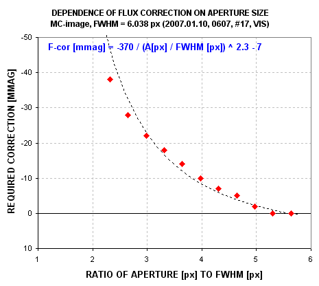
Typical relationship between aperture size and missing flux (flux that's
not captured by the signal aperture).
If R is small the "flux capture fraction" is small, requiring a large "correction." For example, in the above graph if R = 3 × FWHM the measured flux should be increased by ~22 mmag. As seeing varies while R remains fixed this correction will vary. For a telescope with imperfect optics (that includes all telescopes), the size of the point-spread-function, PSF, will vary across the image. The details of this variation will change with focus setting. Therefore, a too small R will produce flux capture fractions that differ across the image, and that change during an observing session. If R is set too large SNR suffers. A large R also increases the likelihood that the signal aperture will contain defects, such as cosmic ray hits or hot and cold pixels due to an imperfect dark frame calibration. A large R also increases the chances that a nearby star will swell in size during bad seeing episodes and contribute some of its flux to the target star's signal aperture. I've seen this last effect cause trends of several mmag. The ideal solution is to employ a "dynamic aperture" such that the image measuring program takes a measure of FWHM for each image and then sets R to whatever multiple of FWHM the user specifies (such as R = 3 × FWHM). Unfortunately, MaxIm DL does not provide this feature yet, and I can't afford to pay them to develop it. (I sometimes perform a "poor man's dynamic aperture" by repeating the readings using a range of R values then later combining them to match FWHM versus time.)
AAVSO observations won't matter if they're affected by a few mmag of systematic
errors. Therefore, if the variable star goal is an accuracy of 0.05 magnitude,
for example, aperture choices are not very important. Simply adopting R
= 3 × FWHM, assuming that all stars suffer the same "missing flux
fraction" (corresponding to ~20 mmag), could allow the observer to believe
that he's dealt with the matter sufficiently. This would be a safe procedure
when systematic errors of ±0.02 magnitude are acceptable, which is
the case for all AAVSO variable star observing tasks. For exoplanet observers
this detail matters.
PRECISION VERSUS ACCURACY
Precision is the consistency of measurements, regardless of any calibration
error shared by all of them. When all calibration errors (systematic errors)
remain constant, precision is given by the Poisson equation: SE = 1/SQRT(N),
where N is the number of discrete events leading to the measured value, N.
Accuracy consists of two components: precision and calibration uncertainties.
Since these two components are uncorrelated (the sign of one is unrelated
to the sign of the other), the two components are added orthogonally. This
means the accuracy uncertainty, SEa = SQRT( SEp2 + SEc2),
where SEp is precision (also called stochastic uncertainty) and SEc is calibration
uncertainty. SEc is almost always subjectively estimated.
In AAVSO related photometry a worthy goal for accuracy is ~0.03 magnitude
(although 0.02 and slightly lower are possible from ground-based observations
if careful procedures are followed). For exoplanet observing, on the other
hand, it is acceptable that a set of observations have an accuracy SE of
0.1 magnitude, or 1 magnitude or even 10 magnitudes! It's totally irrelevant
how accurate an exoplaent light curve is. For AAVSO variable star observing
accuracy is everything, and accuracy SE > 0.1 magnitude is almost never
acceptable. In order to achieve an accuracy of 0.05 magnitude, for example,
it is adequate for precision to be < ~0.02 magnitude (SNR > 50). This
level of imprecision is useless for ALL exoplanet work. No wonder the two
tasks require different strategies for observing and image analysis.
(Uncertainty is stated in terms of SE, standard error, which assumes that
the probability function for a measurement is Gaussian. This, in turn,
permits the use of "least squares" and "chi-square" statistical tools
to be used for fitting measurements instead of Bayesian Estimation Theory,
the "gold standard" for matching measurements with models.)
Return to AXA home page
____________________________________________________________________
WebMaster: Bruce Gary. Nothing on this web page is copyrighted. This site opened: June 28, 2008 . Last Update: July 30, 2008