There are many ways to convert MTP "Observables" to "Retrievables." It will be instructive to review the Backus-Gilbert method, since it illustrates the underlying concepts for all the others.
Consider the weighting functions for a 2-frequency MTP viewing the horizon in a situation where temperature may vary (linearly) with distance along the viewing direction.
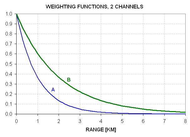
Figure 7.1 Weighting functions for Channels "A" and "B" of a 2-frequency MTP. Applicable ranges are 1.0 and 2.0 km.
For this first example case we may ssume that the weighting functions are exponential since the horizon view guarantees that air density and temperature will be essentially constant versus range. An MTP with weighting functions for Channel A and B having applicable ranges Ra = 1.0 and 2.0 km will measure brightness temperature, TB, corresponding to the temperature of the air at locations 1.0 and 2.0 km away from the MTP (assuming air temperature varies linearly with range).
Now, consider the imaginary weighting function obtained by subtracting one weighting function from the other.
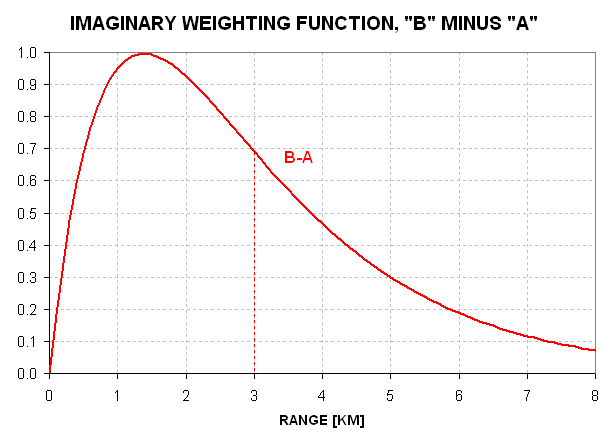
Figure 7.2 Imaginary weighting function obtained by subtracting the weighting functions "A" from "B" and then normalizing to achieve a maximum of 1.0.
The imaginary weighting function in this figure is called an "averaging kernel." If through some magic it were possible to build a radiometer with a weighting function like this averaging kernel the radiometer would measure a brightness temperature equal to the air temperature weighted by the averaging kernel function. Such a TB value would be unaffected by air temperature at the aircraft's vicinity, and would be most-affected by air temperature at ~1.4 km, in the case under consideration. Thi s is in contrast to the TB values for Channels "A" and "B," which are most affected by air temperature in the vicinity of the aircraft and less affected by air temperaature at a range of ~1.4 km. Whereas it is impossible to construct a radiometer with an averaging kernel weighting function, it is possible to derive what such a magical radiometer would measure using the TB measurements of corresponding to channels "A" and "B." This is demonstrated in the next paragraph.
If the "areas" under the weighting functions for "A" and "B" are represented by "a" and "b" then there is something special about the artificially produced observable:
TB_ba = (b/(b-a)) * TB_b - (a/(b-a)) * TB_a
where TB_b = TB for Channel B and TB_a = TB for Channel A
It can be shown that TB_ba is the brightness temperature that would be measured by the magical radiometer with a weighting function corresponding to the averaging kernal.
Let's explore this specific example further, to illustrate how intuitively sensible this result is. The area under "B" is twice the area under "A" since Rb = 2 * Ra. This means that:
TB_ba = 2 * TB_b - TB_a
For example, suppose T(r) = 220 K + 1 [K/km] * r [km]. This corresponds to air temperature increasing with range linearly at the rate of 1 [K/km] starting at 220 K at the origin. For this example TB_b = 222 K, TB_a = 221 K and TB_ba = 223 K. This suggests that the magical radiometer is measruing the temperature at a range of 3 km. Indeed, the calculation of applicable range for the averaging kernel is 3.0 km.
Let's consider what we've done by these simple manipulations of brightness temperatures from a 2-frequency radiometer. We've determined the temperature at 3 ranges:
T(1 km) = TB_a
T(2 km) = TB_b
T(3 km) = 2 * TB_b - TB_a
Of course, each of these inferences is subject to the assumption that air temperature varies linearly with range. Nevertheless, we've demonstrated that it's possible to combine measured observables to infer what imaginary radiometers would measure if they had corresponding imaginary averaging kernels, and the concepts that undely this 2-frequency demonstration can be used with a many frequency radiometer.
The previous analysis was for the situation of an MTP viewing the horizon. What about looking straight up? The only thing that changes is that the atmosphere's absorption coefficient varies slightly with range, which causes the weighting functions to depart slightly from an exponential shape. However, the weighting function shapes can be calculated if the altitude and air temperature at flight level is specified. It may be objected that an accurate calculation of an upward looking weighting function will be influenced by the profile of temperature above the aircraft; this is true, but a first approximation solution can be used to perform a second iteration solution, and if necessary additional iterations can in theory be performed. These second order effects should not distract from the fact that improved solutions for T(z) are possible using averaging kernels.
To implement the Backus-Gilbert retrieval procedure the user must calculate a set of retrieval coefficients for a suite of altitudes, and repeat this for every flight level of interest. Then, for a set of observables at a specific flight level two complete retrievals can be made, one for the flight level above the actual and one for the flight level below the actual, then interpolate the result. The same result is obtained by first interpolating the coefficients and performing one retireval. Typically, a set of 10 flight levels are prepared, and for each flight level a set of 20 or 30 altitudes (above and below flight level) are supported.
The mathematical concepts of improving resolving power by properly combining observables with exponential weighting functions was shown in a paper by Backus and Gilbert (1968). They showed that when many observables are available, corresponding to a large range of applicable ranges, and when the observables have very small levels of measurement uncertainty, it is possible to achieve a resolution corresponding to an averaging kernel a half-intensity ranges of ~80% to 130% of the averaging kernel's applicable range. This performance was not possible at the short and long limits of the averaging kernel applicable ranges, for reasons that should be intuitively obvious. One other interesting result is worth noting: there is no fundamental limit to the range of distances that the Backus-Gilbert retrieval solutions. In other words, if weighting functions for directly measured observables are present for a range of distances (uniformly sampled in a logarithmic sense) that extend from 1 meter to 10 km, a range ratio of 10,000, it should be possible to achieve improved resolution for all ranges withn about 2 meters to 5 km (a range ratio of 2500).
The best-possible averaging kernel, with half-intensity ranges of ~80% and 130% of the averaging kernel's applicable altitude, assume very low measurement uncertainty. In practice, measurement uncertainty is never good enough to achieve the best-possible resolution. A useful rule of thumb is that Backus-Gilbert T(z) solutions correspond to averaging kernels that extend from 60% to 160% of the altitude assciated with the solution. This is still a significant improvement over the "poor man's retrieval procedure."
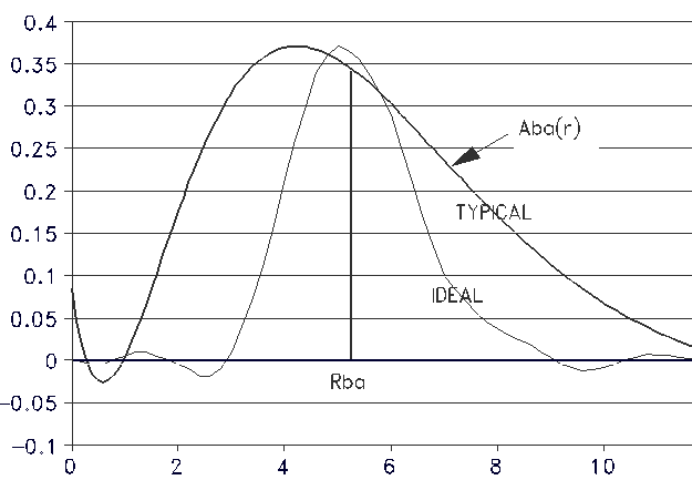
Figure 7.3. Using 8 frequencies with typical measurement uncertainty uses coefficients that correspond to an averaging kernel labeled "TYPICAL" which is not as good as the theoretically possible ideal averaging kernel using many observables with no measurement uncertainty labeled "IDEAL." The two averaging kernels are chosen to have the same applicable range (5.3 km).
The same limitations on altitude resolution are found to apply to all other retrieval procedures that I know about. This is to be expected, since we are dealing with observations with "information" based on the same weighting function multiplied by the same source function, and all retrieval procedures will be subject to the same ambiguities of overlapping "information" associated with a set of observables.
This is illustrated by inspecting the coefficients used by the Backus-Gilbert and statistical retreival procedures. Both are implemented by multiplying each observable with a corresponding coefficient. In the example above, the coefficients for TB_b and TB_a were +2.0 and -1.0. When a larget set of observables are available the coefficients will form a sequence that starts with small values, oscillates and rises to large positive values, then declines and oscilates to small values (I've assumed the observablesa are ordered by their applicable ranges). For both the Backus-Gilbert and statistical retrieval methods the sum of coefficients add up to +1.00, and the plot of coefficient values are quite similar. This is just a reflection of the fact that "information" about the temperature at a specified range is positively correlated the strongest with the observable having the same applicable range, and resolution is enhanced by assigning negative coefficients to observables having nearby applicable ranges. Notice that the Backus-Gilbert retrieval procedure does not assume prior knowledge about likely T(z) profiles. This is both one of its strengths, and also one of its weaknesses, compared to the class of statistical retrieval procedures.
This last paragraph is getting ahead of the story, since I haven't described the statistical retrieval procedure yet. That's done in the next chapter.
Go to Chapter #8 (next chapter)
This is Chapter 7
Go to Chapter #6 (previous chapter)
Return to Introduction
____________________________________________________________________