The previous chapter dealt with the Backus-Gilbert retrieval procedure, which is based on simple manipulations of weighting functions and corresponding manipualtions of observables to arrive at a set of imaginary weighting functions, called averaging kernels, and the brightness temperatures that such averaging kernels would produce. The final step was to assign this hypothetical TB to an applicable altitude corresponding to the hypothetical TB's averaging kernel. The entire procedure had a minimum of assumptions, the principal one being the shape of the weighting function for each observable (frequency and elevation angle of viewing direction). A wide range of assumed temperature profiles would produce a similar set of weighting function shapes, so the Backus-Gilbert retrieval procedure should work in almost any atmosphere regime (tropical, mid-latitude, polar summer, polar winter, etc).
In this chapter we will deal with a procedure that assumes we know what atmospheric regime we are are flying in, and this added information will lead to an increment of performance improvement. However, it is often criticized for biasing the T(z) solution toward an average for that regime, and when an unusual T(z) is encountered its unusual features will be under-represented in the T(z) solution. The user must be alert to this situation, and be prepared to take steps to not be misled. Again, I'm getting ahead of myself; let's describe what the "statistical retrieval procedure" is.
Concepts Underlying Statistical Retrieval Procedure
Consider the hypothetical situation of an MTP flying over many RAOB sites on many dates at altitude Zo. After completing this hypothetical set of observations it would be possible to create a data base of MTP observables associated with each known RAOB-based profile, T(z). The user could then pose the question "If I'm flying at altitude Zo and I want to know the most likely air temperature at altitude Z, how might I use this data base to determine T at Z?" One approach is to perform a multiple regression of T at Z (as the dependent variable) upon the MTP observables (as the independent variables). This could be done using a spreadsheet, for example. The multiple regression solution produces a coefficient for each observable, allowing T (at altitude Z) to be calculated in the following manner:
T = C0 + C1 * O1 + C2 * O2 + ... + CN * ON
where there are N observables (N is typically between 10 and 30). The coefficients are called "retrieval coefficients." The number of RAOB flybys for such an analysis, R, would have to exceed N by a large amount, and it is generally recognized that R must exceed ~100 to assure that the coefficients Ci are useful.
In order to derive T for another altitude the above procedure could be repeated. If there are L altitudes for which coefficients are calculated then there will be a N x L matrix of coefficients that can be used to calculate a profile of T(z) for L discreet altitudes.
For flight at another altitude the entire procedure, above, would have to be repeated. When this has been done for a range of altitudes, such as 6, 8, 10, ... 20 km, the collection of retrieval coefficients for all flight altitudes can be referred to as a "retrieval coefficient set." A retrieval coefficient set obtained in this way would be useable for flight at any altitude for future flights provided the flights were made in the same geographical region during the same season. Henceforth I shall use the term RCs to mean "retrieval coefficients" and also "a retrieval coefficient set."
Clearly, it is not feasible to fly in a specific area during a specific season for the hundreds of hours needed to obtain several hundred cases of simultaneous RAOB data simply to be prepared for the science flights at that location and season. Instead of using actual MTP observations as input to the multiple regression analyses it is possible to use "calculated observables." This oxymoron-sounding terminology is not misleading, since it should be possible to calculate what a perfectly calibrated MTP would observe if it were placed at a specified altitude in an atmosphere with T(z) given by a RAOB. This, in fact, is a practical way for deriving RCs.
Dealing With Stochastic Uncertainties and Systematic Errors
It is impossible to achieve a perfect calibration of any radiometer. Fortunately, there's a way to allow for an imperfectly calibrated MTP when calculating RCs. The process can best be described using matrix terminology, which I will not do in this web page. I will merely state that an "error matrix" can be created (the diagonal elements of an N x N array are used to specify estimated systematic uncertainties for the N observables), and this matrix is added to an auto-covariance matrix of the observables before it is inverted, etc. The matrix manipulation procedure which I will not describe is equivalent to repeating the perfect MTP calculation of RCs many times, where each time the perfect observables have been altered in a stochastic manner that simulates systematic uncertainties.
Even if the MTP were perfectly calibrated it is still subject to a stochastic component of noise on each observable. This stochastic component of observable uncertainty is usually less important than the systematic error component, but there is a way to allow for it when calculating RCs. Usually the two components (stochastic and systematic) are "lumped together" (orthogonally added) and treated in the manner alluded to above.
This completes my description of the "statistical retrieval" procedure. It has emphasized underlying concepts instead of procedural steps. Additional procedural information can be found in many places, including my Rockwell tutorial web page http://brucegary.net/RKW/. Also, Dr. M. J. Mahoney has become expert in many sophisticated versions of the statistical retrieval procedure and I prefer to refer the reader to his web pages on this subject (when they become available).
Comparison with Backus-Gilbert
It is interesting to compare the values of statistical RCs with the values of corresponding Backus-Gilbert coefficients. Recall that both approaches make use of the same expression for calculating temperature at a specific altitude: T = C0 + C1 * O1 + C2 * O2 + ... + CN * ON. When the coefficient values are ordered by their associated observable's applicable altitude both plots are similar. As shown in the next figure the coefficient values typically start out small in absolute value, then go negative before abruptly growing to high positive values in the region corresponding to the observable that contains the most "information" about the altitude in question, then decrease and go negative, then oscillate above and below zero to vanishing small values. This intuitively expected behavior is just a restatement of where information resides among the series of observables for the altitude under consideration. The presence of negative regions astride the main positive region simply means that the statistical retrieval procedure leads to retrieved T(z) that has sharper structure features than the "simplest possible" procedure described in Chapter 6 - in which TB(Ra) is converted to T(z) by assuming T = TB and z = Zo+Ra*sine(theta). The advantage of the statistical retrieval over Backus-Gilbert is that it is easier to calculate RCs.
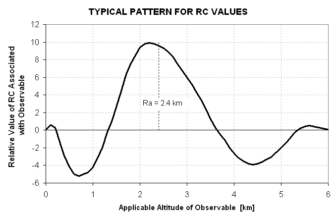
Figure 8.1. Typical shape of RC values plotted versus the applicable altitude of the associated observable. This RC sequence is for retrieving temperature at an altitude of 2.4 km.
There's another property of the statistical retrieval procedure that should be kept in mind. Since it involves finding a solution that minimizes the RMS of residuals (in observable space) it will produce solutions that tend to resemble the average of the RAOBs used in the simulation archive. This is both a strength and a weakness of the statistical retrieval procedure. It is a strength when flying though air that resembles the archive, but it is a weakness when flying though air that differs from the archive. In other words, when a rare but significant atmospheric situation is encountered the simple statistical retrieval procedure is likely to produce T(z) results that are inferior to a Backus-Gilbert based retrieval. Fortunately, the statistical retrieval user has a way to recognize this situation, and recovering from naievely accepting a misleading result. It involves comparing observables with the archive average observables, and when they differ by more than some subjective threshold an automatic search for a new set of RCs can be performed. This is a strength of the statistical retrieval procedure in which Dr. Mahoney has become expert.
The next chapter describes ways to overcome the limitations of the statistical retrieval procedure by 1) stratifying RCs, 2) trial and error RC selection, and 3) calulation of RCs based on a post-mission selection of RAOBs resembling those encountered during the mission. The chapter after that describes a totally new procedure, a search for the best fit within an immense data base of pre-calulated observables for selecting T(z). It also describes a "mutation and evolution" retrieval procedure that is very amusing for its oddity.
Go to Chapter #9 (next chapter)
Go to Chapter #7 (previous chapter)
Return to Introduction
____________________________________________________________________