The question of "what's the MTP resoultion, both in altitude and horizontally?" occasionally arises. The last chapter describes altitude resolution; this chapter describes horizontal resolution.
We shall adopt the same MTP and observing setting to illustrate the concepts of calculating horizontal resolution; namely, an MTP/ER2 flying at 20 km in a standard atmosphere. Channel #1 (LO = 56.65 GHz) observes an atmosphere with a microwave absorption coefficient, Kv = 0.39 Nepers/km, corresponding to an applicable range of ~2.6 km. Channel #2 (LO = 58.8 GHz) observes an atmosphere with a microwave absorption coefficient, Kv = 0.9 Nepers/km, corresponding to an applicable range of ~1.1 km. An observing cycle consists of switching between each frequency at each of 10-elevation angles. The elevation sequence is +60.0, +44.4, +30.0, +47.5, +8.6, 0.0, -8.6, -20.5, -36.9 and -58.2 degrees. The next three graphs are similar to those ones in Chapter 6, but they have been calculated for the specific case under discussion in this chapter.
If the ER-2 were not moving through the air the applicable ranges for each channel, at each of the 10 scan angles, could be depicted by the following graph.
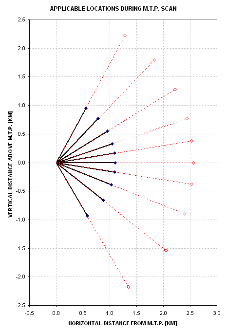
Figure 13.01. Applicable range locations for a 2-channel MTP that is not moving through the air as it completes an elevation scan. The elevation angle sequence and applicable ranges are given in the text.
Since the ER-2 is moving at 210 meters/second the applicable locations of a scan are offset as shown in the next figure.
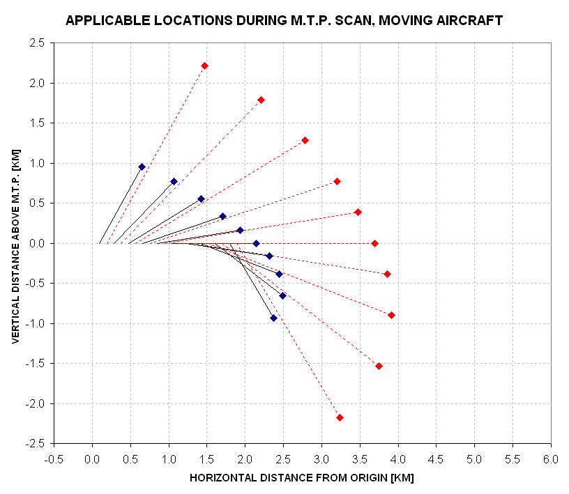
Figure 13.02. Applicable range locations for a 2-channel MTP that is not moving through the air as it completes an elevation scan. The scan direction is downward.
Elevation scan sequence are 10 seconds apart so the air sampled by one scan cycle is 2.1 km offset from the air sampled by the previous scan cycle - as shown in the next figure.
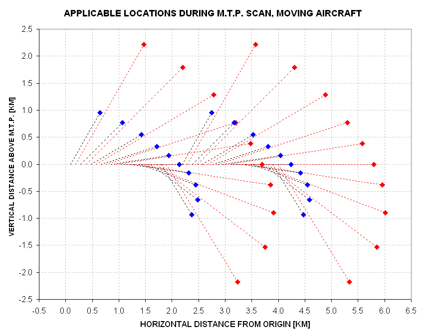
Figure 13.03. Applicable locations for two MTP scan cycles (for cycle spacing of 10 seconds).
Remember that each applicable location symbol is just the 1/e location of an exponential weighting function. For the horizon views (scan location 6 for each channel) the weighting functions for two scan sequences is shown in the next figure.
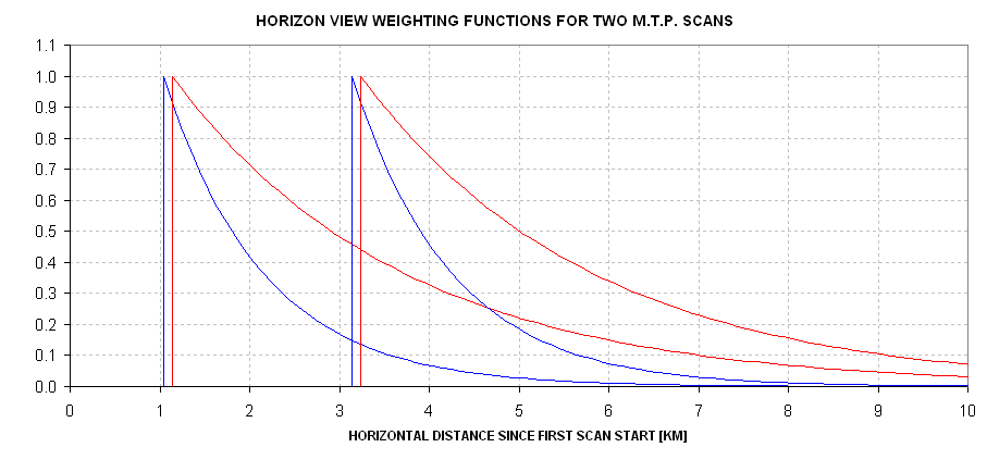
Figure 13.04. Horizon view weighting functions for two scans, for Channel #1 (red) and #2 (blue).
Now we're ready to give a first approximation answer to the question "What's the horizontal resolution of MTP temperature profiles?" Our answer will apply to the MTP-based OAT at flight level, called OATmtp. Assuming Ch #1 and Ch #2 horizon view brightness temperatures, TB1 and TB2, are weighted equally for the calculation of the parameter OATmtp (outside air temperature based on MTP), each elevation angle scan cycle's OATmtp comes from a quasi-exponential weighting function shown in the next figure.
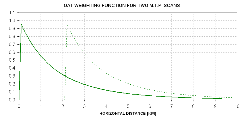
Figure 13.05. OATmtp weighting function (the average of horizon view weighting functions for Ch #1 and Ch #2). The next cycle's weighting function is shown by the dotted trace.
The 1/e distance of the OATmtp weighting function = 1.8 km. This is approximately the same as the spacing of neighboring OATmtp weighting functions (2.1 km). It is tempting to say that horizontal resolution is ~2 km. But there's the matter of undersampling. If TB measurements of the horizon were made twice as often then we could be confident of the 2 km resolution answer. Let's look at the matter of horizontal resolution differently.
Fourier Representation of T(x)
The term "resolution" will have different meanings for observing systems having different weighting functions. For example, an in situ sensor reading is actually the weighted average of the source function, T(x), multiplied by an exponential function that tails off behind the aircraft with a distance of tens of meters. The e-folding distance for the MMS in its low resolution mode is ~200 meters. An MTP reading of brightness temperature, on the other hand, is the product of T(x) multiplied by an exponential weighting function that tails off in the opposite direction (assuming the MTP views the horizon in the direction of flight). Even if the OAT sensor and the MTP had the same e-folding distance, and same measuring interval, they would have different observable sequences. In theory, however, it should be possible to reconstruct the same source function, T(x). This would be done using a Fourier component representation of the observations and reconstructing the source function by shifting component phases in an appropriate manner.
An observing system can be imagined that does not have an exponential weighting function. For example, consider representing T(x) by the function 2 * TB2 - TB1, where TB1 and TB2 are the MTP Ch#1 and Ch#2 brightness temperatures for the horizon view. This is a simple Backus-Gilbert procedure for improving horizontal resolution; it is the horizontal analogue of the vertical resolution improving procedure described in the previous chapter (see Fig. 12.10). The location x where this temperature applies is ahead of the aircraft's position, and the distance correction is merely the applicable range of the averaging kernel times airspeed.
I'm not suggesting that this procedure be used for converting MTP measurements to T(x); rather, I'm using it to illustrate that an exponential weighting function is not the only one to describe observations that are to be used in deriving T(x). When someone asks "What's the horizontal resolution of your measurement?" you have to ask "How do you want to define 'resolution'?"
Let's work-up to a suggested definition in steps. Consider that the observations can be used to derive a most-likely source function, T'(x). A first approximation to T'(x) is merely:
T(x+Ra) ~ T'(x+Ra) = TB(x) (1)
where TB is measured brightness temperature while flying at location x, and
Ra is the applicable range corresponding to the TB observable.
Four equally-spaced measurements (thanks, MJ) are needed to measure a sinsoidal funtion's amplitude and phase (at, for example, phase = 0, 90, 180 and 270 degrees). Therefore, the shortest wavelength that can be represented by TB(x) is ~8.4 km (4 x 2.1 km), assuming TB measurements are made every 2.1 km along the flight path. Longer wavelngths can be represented, the longest being set by the length of the TB sequence.
It will be useful to now consider the response of an MTP to Fourier components of the source function T(x+Ra) with the weighting function geometries for our case study MTP.
First, recall that the MTP's estimate of OAT is obtained by averaging the horizon brightness temperatures for two (or three) channels. The weighting does not have to be equal, and in the past the weighting has been influenced by the RMS performance of each channel. Whenever a weighting is performed the effective weigting function versus range is no longer an exponential. The following figure is a plot of the weighting functions for a set of 6 TB measurements of the horizon view (using the same shape as in the previous figure).
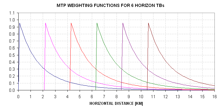
Figure 13.06. Weighting functions for a set of 6 MTP OAT estimates.
The set of 6 measured TBs are obtained by multiplying these 6 weighting functions with the source function T(x).
Now, think of the true source function, T(x), as consisting of Fourier sine and cosine components with wavelengths corresponding to all relevant spatial frequencies. Let's start with a T(x) sinusoidal component having a wavelength of 12 km.
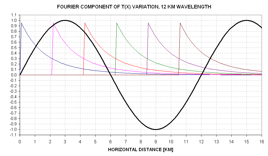
Figure 13.07. 12 km wavelength Fourier component of T(x), air temperature along the flight path, T(x). The y-axis can be thought of a a Kelvin scale for the Fourier component.
Using this graph it can be seen that the MTP's OAT response to a 12 km wavelength component of variation in T(x+Ra) appears to be close to 100%. A detailed calculation (involving sliding the sequence of weighting functions in phase to get the maximum response) shows that the maximum observed TB variation is 68% of the true source variation. Thus, the function TB(x) has a 68% response to Fourier components with a 12 km wavelength. Similar calculations for other wavelengths have been made, and are plotted in the next figure.
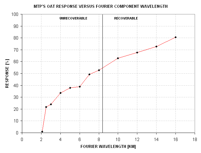
Figure 13.08. Response of MTP's OAT versus Fourier wavelength of T(x) function.
What is the meaning of the non-zero response shortward of 8.4 km (which is the shortest wavelength for which we can derive Fourier components for the desired source function)? The non-zero response to short wavelengths should be viewed as "noise" cased by real T(x+Ra) variations whose Fourier components cause TB fluctuations but whose amplitudes and phases we cannot recover. This is a problem related to having weighting functions with an abrupt "turn-on" near the aircraft.
Since the weighting function width for each averaged horizon view TB is slightly shorter than the sampling distance there will be additional "noise" for Fourier components near 8.4 km. If the Ch#1 TB were used by itself to create a TB(x) sequence then there would be less noise near 6.3 km due to real T(x+Ra) structure with wavelengths shorter than 8.4 km.
Lest we forget, I should mention that there's another component of noise that will limit horizontal resolution, and that's radiometer noise. Any analysis done with the observed TB sequence for the purpose of recovering T(x+Ra) will have to take into consideration the stochastic noise on each TB measurement, which is ~0.2 K.
If no attempt is made to recover T(x+Ra) structure from TB(x) then it can be said that the MTP's horizontal spatial resolution is ~2 km, corresponding to a highest spatial frequency that can be represented by the function "true air temperature versus distance along the flight path" of ~ 8 km. Due to undersampling this resolution is subject to some additional "noise" caused by T(x+Ra) structure with wavelengths shorter than 8 km.
Deconvolution
This web page's objective is to answer the question "What's the MTP's horizontal resolution?" Nevertheless, this is a good place for describing how the observed set of TB(x) measurements (actually, the average of Ch#1 and Ch#2 TB measurements) can be used to produce improved T(x+Ra) solutions. We will conclude that this is an unworthy goal.
There are at least two methods for attempting to recover a better version of T'(x+Ra) than by assuming it to be TB(x). The simplest of them is Bracewell's deconvolution method. You begin with TB(x) as a first approximation of T(x+Ra) and then pretend to observe it. The fictitious observation sequence will have less structure than TB(x), and the difference between the two sequences is the first iteration correction to TB(x). Each iteration multiplies the effect of stochastic noise, so when the corrections become comparable to, or smaller than, the noise level of the TB observations you terminate the process. The Bracewell deconvolution is almost equivalent to multiplying the high spatial frequencies in the observations by their lowered response to true variations of high spatial frequency.
Another method for recovering structure is to choose an x-region of interest and decompose the series TB(x) into Fourier components. This will be done using spatial frequencies (not wavelengths). The minimum spatial frequency will be Fn = 1 / (2 * L), which is also the spatial frequency interval, dF, and the maximum spatial frequency will be (N-1) * Fn - where L is the length of the data set, and N is the total number of evenly-spaced TB data. Windowing should be performed first (my favorite is Welch). After calculating the entire set of N-1 sine and cosine amplitudes the amplitudes should be adjusted upward in accordance to Fig. 13.08 (i.e., using the reciprocal of the response as multipliers). The amplitude adjusted Fourier components should then be added to produce a new T'(x+Ra). The new T'(x+Ra) will have the shorter wavelengths of temperature variation restored. Unfortunately, the "noise" produced by wavelengths that cannot be recovered (see previous figure) will be amplified as they show themselves as spurious fluctuations at the short wavelength end of what can in theory be recovered. This problem originates in the weighting function having a sharp "turn on" near the aircraft. The only way to overcome this problem is to use a horizon view version of the Backus-Gilbert averaging kernel shown in Fig. 12.10 and 12.11. These B-G averaging kernels have "soft" shapes and they therefore will not have "noise" produced by fluctuations shorter than can be used in a deconvolution process. The only downside to this is radiometer noise. The B-G procedure multiplies radiometer noise, as does the Fourier deconvolution procedure. When each TB reading, for each channel, has a stochastic uncertainty of ~0.2 K, the final deconvolved T'(x+Ra) will have stochastic SE on the order of 1.0 K. I therefore do not recommend using any of the structure recovery procedures for horizontal temperature.
Suggested New Equation for OATmtp
Considerations of the previous few paragraphs suggest that a new way be used for computing OAT from MTP measurements:
OATmtpNew = 2 * TB1 - TB2 (2)
where TB1 is Ch#1's horizon view TB, and TB2 is Ch#2's horizon view TB.
The following figure shows the shape of the averaging kernel for "OATmtpNew":
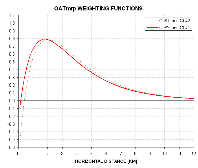
Figure 13.09. Averaging kernel for OATmtpNew = 2 * TB1 - TB2 for two frequency switching choices.
The slight difference timing for the TB1 and TB2 measurements causes a negative feature at the beginning of the OATmtpNew's averaging kernel. The next figure shows the weighting functions for the frequency swtiching sequence "Ch#2 then Ch#1."
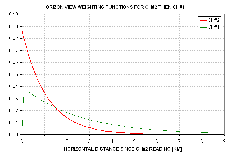
Figure 13.10. Weighting functions for Ch#2 before Ch#1 (horizon view). Ch#2 "turns on" at the origin while Ch#1 "turns on" ~0.1 km later.
Since the two measurements are made ~0.4 seconds apart (~80 meters of difference along the flight path) only temperature fluctuations on this scale will produce spurious, high spatial frequency artifacts in OATmtp. These fluctuations are miniscule in comparison to those that affect the old version of OATmtp. The only disadvantage in using OATmtpNew is that the stochastic noise per 10-second observing cycle will be ~0.5 K instead of 0.2 K.
Notice that it is better to observe Ch#2 before Ch#1 at the horizon view scan location since that frequency order produces a slightly better averaging kernel shape. The FWHM for the "Ch#2 then Ch#1" averaging kernel is 4.2 km. This is twice the interval between samples; this means that using the new OATmtp equation there is no undersampling problem. In fact, a sequence of OATmtpNew has the potential for a proper deconvolution since its sampling meets the Nyquist requirement.
In conclusion,
The MTP's horizontal resolution is ~2 km near flight level but the readings are undersampled by about a factor two. At 1 or 2 km above and below flight level the horizontal resolution is about 2 to 3 km, and the same undersampling exists. For all previous calculations of OATmtp a component of high spatial frequency fluctuations is present because the observables have exponential (non-Gaussian) weighting functions with a sharp turn-on shape near the aircraft; this produces observables that are influenced by temperature fluctuations having wavelengths shorter than the stated resolution. A new equation for calculating OATmtp is suggested which does not suffer from this problem; it has a horizontal resolution of 4.2 km but because it meets the Nyquist sampling requirement it may be possible to achieve a somewhat better horizontal resolution, such as ~3 km.
Go to next Chapter #14
Go to previous Chapter #12
Return to Introduction
____________________________________________________________________