Occasionally someone asks "What's the MTP resoultion, both in altitude and horizontally?" This chapter describes altitude resolution; the next chapter describes horizontal resolution.
This chapter has three sections: 1) horizon staring, 2) elevation scanning and near flight level altitude resolution, and 3) elevation scanning and far from flight level altitude resolution. With this structure we can deal with simple concepts first, making them available for the more difficult problems.
Horizon-Staring MTP
Imagine fixing the MTP's viewing direction to the horizon and taking measurements at one frequency. Let's assume that the antenna pattern has a HPBW (half-power beam-width) of 7.5 degrees. Let's also assume that the atmosphere's microwave absorption coefficient, Kv, is 0.9 Nepers/km (corresponding to the LO = 58.8 GHz while flying at 20 km in a standard stmosphere).
Now we are ready to ask "For this observing situation what is the altitude resolution of each observation?"
We begin by noting the antenna pattern.
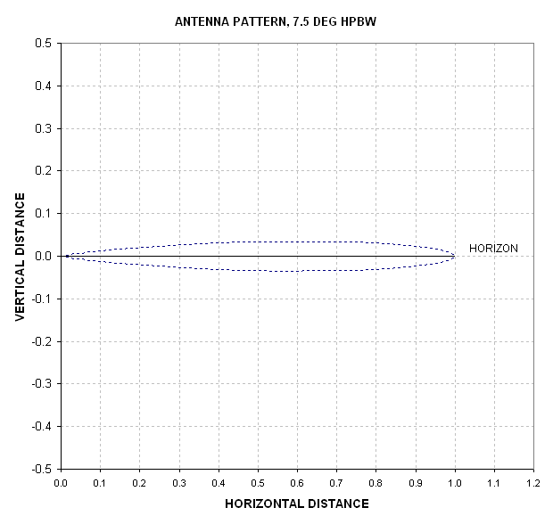
Fig. 12.01. Antenna pattern for HPBW = 7.5 degrees, to scale, when viewing the horizon. The MTP is located at the origin (0,0) and the antenna response in any direction is proportional to the length of the line from the origin to the dotted pattern in that direction (see next figure for another representation).
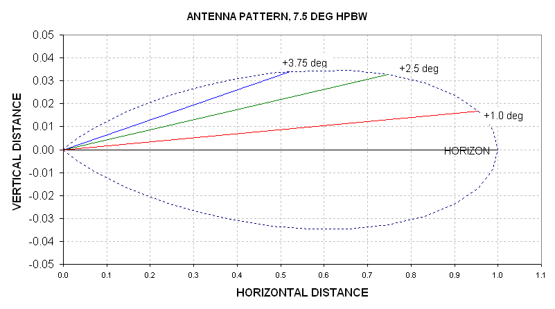
Fig. 12.02. Antenna pattern with a 5x vertical expansion.
In this last figure notice that the antenna response at an angle +3.75 degrees is about half the horizon response; that's what it means to have a HPBW = 7.5 degrees. Also keep in mind that the antenna pattern is circularly symmetric. As it turnsout, this won't matter, but it's an issue we'll come back to later.
This way to represent an antenna pattern may be confusing. The length of the line to the antenna pattern dotted line is merely the relative response for radiation arriving from that direction. Radiation from all distances have a finite probability of arrivng at the MTP location and entering the antenna, but the probability function scales with the response for that direction (i.e., the length of the line). Let's think about this situation using a different diagram.
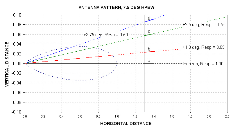
Fig. 12.03. Antenna pattern response in different directions (X and Y ranges shown are twice that of previous figure). The vertical lines at x = 1.3 and 1.4 km represent a vertical slab of air (paralle to the picture plane) for which we want to calculate a contribution to measured antenna temperature, specifically from regions "a" through "d".
In this figure we show four elevation angles and their corresponding antenna response values (normalized to the maximum response at beam center). For example, photons emitted by region "c" have a probability of being received by the horn antenna that is only 75% of that for photons emitted by region "a". In this diagram, with the vertical scale expanded by a factor five, it looks like the picture plane is farther from the antenna at the +2.5 degree intersection location (region "c") than the horizon location (region "a"); however, it is actually only 1.0009 times farther away. For simplicity we will assume that the distances for all picture plane intersections are the same. That means that photons emitted at "c" are 75% as likely to be received by the antenna as the photons from "a" (this implicitly assumes that the distances to these radiating regions is the same, so that the intervening absorptions are the same).
The altitudes of these four emitting regions are given by "range" times "sine theta" (where theta is the elevation angle). The range for this example is 1.35 km (or 1.30 to 1.40 km). The relative contributions of photons received versus altitude is simply a Gaussian function with a FWHM (full-width half-maximum) specified by the following simple equation:
FWHM of Altitude Contributions to Ta = 2 * tangent (7.5 degrees / 2 ) * Range Eqn 12.1
where we are adopting the proportionality of photons received with contribution to antenna temperature, Ta.
So far all we've shown is that considering a slab at a known range we can easily calculate the altitude resolution, or a FWHM version of altitude resolution, for the emission received by the MTP antenna. OK, I know that you're now wondering about the fact that the antenna pattern, as viewed from the MTP, has circular symmetry. It's time to invoke a well-known mathematical property of 2-dimensional Gaussian functions: considering an intensity (z-axis) of a Gaussian centered at x,y = 0,0 that has a Gaussian shape versus x, and a Gaussian shape versus y, the shape of intensity versus any straight line in the x/y plane is another Gaussian; moreover, if the Gaussian is circularly symmetric (same FWHM in x and y), then all intensity versus location along straight x/y lines are Gaussian with the same FWHM. If you didn't know this, then it would be a good homework assignemnt to prove it to yourself. I can provide a proof if you get stuck.
Invoking this neat little Gaussin properties trick means that if you consider an azimuth offset from beam center, and ask what the shape is for emission versus altitude at this offset azimiuth, the answer is that the shape is Gaussian with the same altitude FWHM, merely reduced in scale (i.e., multiplied by a number less than one and corresponding to the intensity of the Gaussian at he horizon at the offset azimuth). Sorry if all this is too simple, and you already know it, but I don't want to leave out steps for the person unfamiliar with Gaussian antenna patterns.
We've just shown that the altitude resolution for a 2-dimensional Gaussian antenna pattern that is receiving emission from a picture plane slab at a specified range is given by Eqn 12.1, above. This is not the altitude resolution for the MTP because we have not yet considered emission from all ranges. That's the next step.
Recall that because of interveneing air that absorbs some of the more distant photons the resultant function for where emission comes from (that's received by the horn antenna) is an exponential function. The 1/e-range, called the applicable range, is simply 1/Kv, when Kv is uniform versus range. To calculate an MTP's altitude resolution we must do some integratral math. Define A(r) to be the altitude FWHM resolution as a function of range (eqn 12.1). Define Le to be applicable range, 1/Kv. Then the range-weighted altitude resolution is:
A = Integral { A(r) * W(r) * dr } / Integral { W(r) * dr } Eqn 12.2
where W(r) is a weighting function, EXP( - r / Le ).
Now we can make use of a property of exponential weighting functions: the weighted average vallue of a source function versus range r that varies linearly with r is simply the value of that function at the weighting function's 1/e distance. We've already shown that A(r) is proportional to range, r. So, the value for A is simply A (r = Le). In other words,
A = ( 1 / Kv ) * 2 * tangent ( HPBW / 2) Eqn 12.3
If Le = 1 / 0.9 = 1.1 km (consistent with our assumed Kv = 0.9 Nepers/km), then A = 1.1 [km] * 2 * tangent (7.5 degrees / 2). Or, A = 0.131 km.
For someone experienced with radio telescopes all of the above can be done in about 10 seconds with a hand calculator. There's nothing controversial in this derivation. Sorry to burden you with so much detail.
Let's pause and restate what we've done. We've shown that an MTP that stares at the horizon has an altitude response that is Gaussian if that's the shape of its antenna pattern, and that this "altitude source function" has a Gaussian FWHM (i.e., the altitude resolution) given by eqn 12.3. It is possible to achieve better altitude resolution by observing at elevation angles slightly different from the horizon. That is topic for the next section of this web page.
Elevation Scanning for Improved Altitude Resolution Near Flight Level
First I want to convince you that by scanning in elevation it is possible to improve altitude resolution.
Consider the case of a 1-dimensional reception pattern that is observing a 1-dimensional source function that has structure at all spatial frequencies. Theoretically, it is possible to recover Fourier components of the source function if the reception pattern has the same Fourier components. Signal-to-noise is one practical limitation; so is an imperfect knowledge of the reception pattern (i.e., the amplitude and phase of each Fourier component of the antenna pattern). In practice a two-fold improvement in resolution is achievable. In other words, if the antenna pattern is a Gaussian with HPBW = 7.5 degrees, with sufficient signal-to-noise and knowledge of the antenna pattern it should be possible to recover structure having FWHM ~ 4 degrees. In the example of the previous section an altitude resolution of ~70 meters should be achievable.
Note two assumptions that don't strictly apply to a typical MTP: 1) the elevation scan sequence undersamples the potentially observable function Tb(EL), and 2) for angles that are inclined to the horizon the shape of the altitude response function departs from the antenna pattern projected onto the picture plane at the applicable range. Referring to the first point, it would be necessary to sample at the Nyquist interval of 1/2 times HPBW in order to recover the source function structure to the levels mentioned in the previous paragraph. Instead of sampling elevation angles 0, 4, 8, etc, an MTP is typically sequenced through elevation angles whose spacing is about twice as great (i.e., 0, 8, 16, etc). This is done in order to complete a scan in a reasonable time (10 to 15 seconds). Referring to the second point, whereas at the horizon the altitude response function (for observables) is Gaussian, at zenith and nadir, for example, the response functions versus altitude are exponential. At intermediate elevation angles the altitude response functions (for observables) will be intermediate between Gaussian and exponential. We'll demonstrate this in this section.
For altitudes that are far from flight level, and when statistical retrieval procedures are employed, the altitude response function for the "averaging kernels" somewhat resembles a Gaussian centered at the altitude for which a retrieved air temperature is made (see Chapter 8, Fig. 8.1 for an example). This will be demonstrated in the next section of this chapter.
Now, let's ask "What is the weighting function for observables near the horizon (but not at the horizon)?" Consider the case of EL = +8.6 degrees.
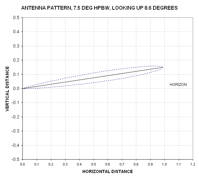
Figure 12.04. Beam pattern for +8.6 degree elevation angle view.
If the antenna pattern is considered to consist of a finite number of components, then each component's line-of-sight will be inclined to the horison. Therefore, each component will have an associated altitude weighting function that has an exponential shape. To perform a calculation of each of these shapes, which will be followed by a weighted average, it is necessary to represent the antenna pattern using a small number of components, as depicted in the following figure.
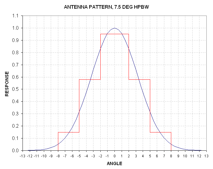
Figure 12.05. Five-component representation of the antenna pattern.
Each of these 5 components has its own altitude weighting function, as shown in the following figure.
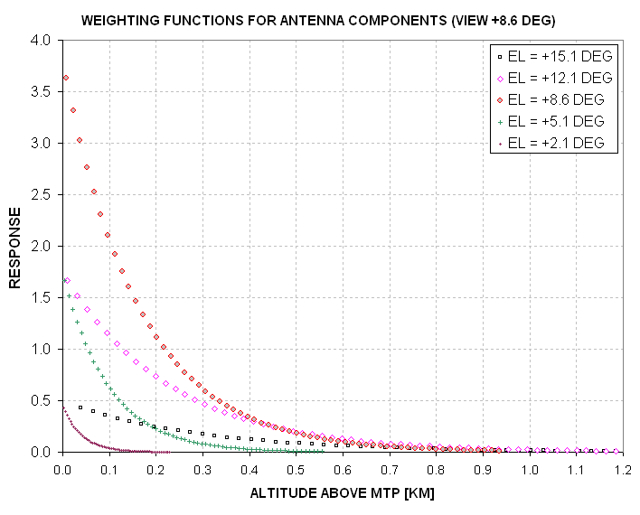
Figure 12.06. Five-component weighting functions versus altitude. The legend shows elevation angles.
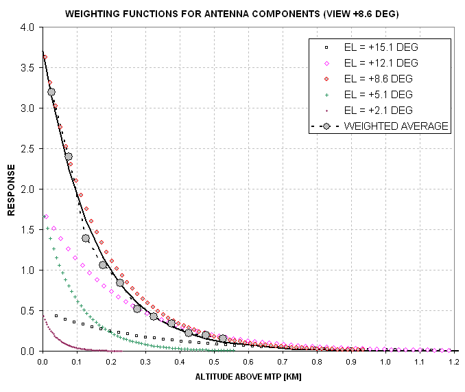
Figure 12.07. Five-component weighted average "altitude weighting function" for the +8.6 degree view.
This graph shows the altitudes which contribute to the observable (measured Ta) for the +8.6 scan elevation as constructed from a 5-component representation of the antenna pattern. The 5-component weighted average altitude plot resembles the beam center component in having an exponential shape with a 1/e distance of 0.15 km. It is therefore safe to adopt the beam center weighting function for all scan angles above 8.6 degrees, and below -8.6 degrees. This simplifies subsequent derivations.
Let's compare the altitude sampling for the horizon view and +8.6 degree view.
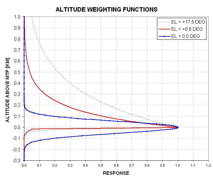
Figure 12.08. Altitude weighting functions for observables at three elevation scan locations.
The following list summarizes altitude weighting function properties for three scan locations:
EL ApplicableAlt FWHM FW37% Shape
+17.5 deg 310 meters 230 meters 370 meters exponential
+ 8.6 deg 140 meters 110 meters 150 meters exponential
+ 0.0 deg 0 meters 130 meters 154 meters Gaussian
Notice that altitude resolution is best at +8.6 degrees if the FWHM criterion is used. However, if a "full-width at 37% response" criterion is used the horizon view is best. I've highlighted the 37% widths because I think these are a better way of specifying altitude resolution than FWHM. Notice that for this set of three scan locations the applicable altitudes have a spacing of about 150 meters, and this is approximately the same as the altitude resolution. What's true for the two scan locations above the horizon will also be true for the two scan locations below the horizon, at -8.6 and -20.5 degrees. Therefore, we can state the following:
EL ApplicableAlt FWHM FW37% Shape
+17.5 deg 310 meters 230 meters 370 meters exponential
+ 8.6 deg 140 meters 110 meters 150 meters exponential
+ 0.0 deg 0 meters 130 meters 154 meters Gaussian
- 8.6 deg 140 meters 110 meters 150 meters exponential
-20.5 deg 310 meters 230 meters 370 meters exponential
To summarize this table, within the 600 meter region centered on flight level there are 5 observables with applicable altitudes evenly spaced at ~150 meters, and they have weighting functions affording altitude resolution of ~150 meters within the 300 meter region centered on flight level. Stated another way, the MTP observables afford an altitude resolution of ~150 meters within a 300 meter altitude region centered on flight level. For altitudes beyond 300 meters the observables exhibit worse altitude resolution.
For altitudes farther from flight level than ~200 meters (for flight at 20 km) there's a better way of assessing altitude resolution of retrieved air temperature than the method used in the preceding few paragraphs. Each retrieved air temperature is derived by multiplying observables by their corresponding retrieval coefficients. The resultant temperature is equivalent to "the averaging kernel weighted average of the actual air temperature profile." This means that if we view the averaging kernel associated with each retrieved air temperature we will be viewing a graph showing the altitude resolution in complete detail. The averaging kernel is calculated by summing the observable weighting function profiles multiplied by their associated retrieval coefficient for the altitude under consideration. Let's demonstrate this with a simple example (which repeats some of the material in Chapter 7).
Consider the weighting functions for the Ch#1 observables for EL = +8.6 and +17.5 degrees.
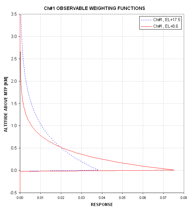
Figure 12.09. Observable weighting functions for Ch#1 EL = +8.6 and +17.5 degrees, normalized so that the integral equals one (for the altitude spacing chosen).
The meaning of an observable weighting function is quite simple: the product of the observable's weighting function times the source function (temperature profile in this case) is equal to what's observed. This was explained in Chapter 7. Consider the hypothetical weighting function defined as C = 2 * B - A, where B refers to the EL=+17.5 degree observable weighting function and A refers to the EL=+8.6 degree weighting function. The weighting function for C is shown in the next figure.
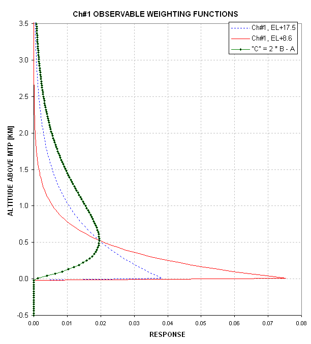
Figure 12.10. Hypothetical weighting function "C" (green) obtained by combining observable weighting functions "A" and "B" (where A = EL+8.6, B = EL+17.5).
If an MTP could somehow observe with the weighting function "C" the observed brightness temperature would be for an altitude region that has better altitude resolution than for either "A" or "B". In fact, an MTP can predict what would be observed if it had an observable weighting function "C"; this fictitious observed brightness temperature is simply TB_C = 2 * TB_B - TB_A. The green trace is called an "averaging kernel", and an averaging kernel can be thought of as sharing the property of a n observable weighting function since: TB_C = sum of products (Averaging Kernel for "C") * (source function T(z) ). The applicable range for this particular simple averaging kernel is 1.14 km. This is a simple Backus-Gilbert retrieval.
Notice that the averaging kernel provides a complete description of the altitude resolution for the "retrieved" air temperature (z = 1.14 km for this example). The peak response is at an altitude closer to the observer than the retrieved altitude. This is always the case for a Backus-Gilbert retrieval.
I will leave it to the reader's imagination that an averaging kernel can be "sharpened" by including more observables, as illustrated by the following graph.
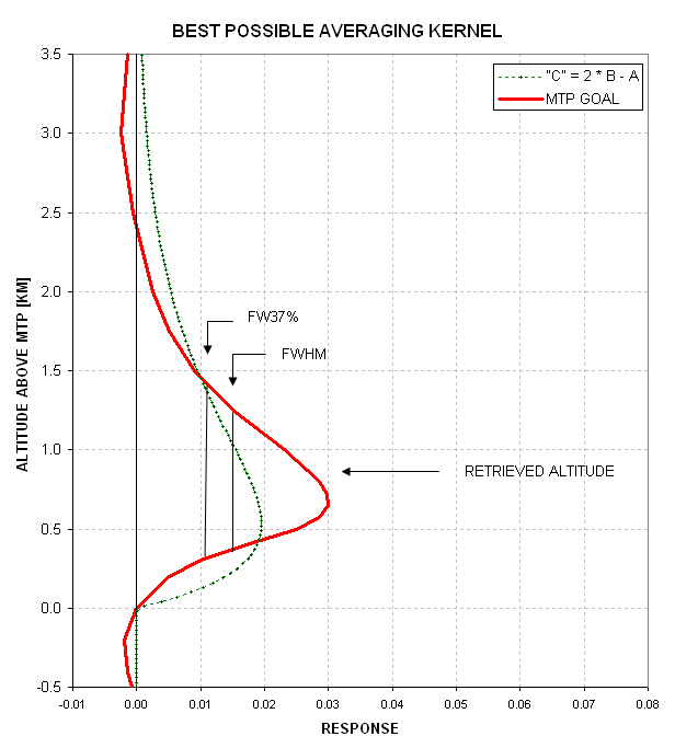
Figure 12.11. Example of a good MTP averaging kernel shape (artistic rendition). The half response altitudes are at ~50% and 150% of the peak response altitude (and ~60% and 160% of retrieved altitude).
The rule-of-thumb for averaging kernel shape for an MTP with many observables (covering a wide range of applicable altitudes with a spacing of approximately 1.5 to one for all nearest neighbors) is that the averaging kernel response is at half-maximum at altitudes that are ~60% and ~160% of the peak response altitude. This is only true when the observed quantities exhibit a high signal to noise ratio (SNR) and have been well-calibrated (to remove systematic errors). This is equivalent to saying that the FWHM resolution for a well-retrieved air temperature can be no better than the altitude under consideration.
Classical Backus-Gilbert theory states that if there is an almost unlimited number of properly chosen observables, all perfectly calibrated, it is possible to create averaging kernels with half response altitudes of 70% and 140% of the peak response altitude. This performance will never be achieved by an MTP.
The term "between penultimate altitudes" is important for statistical retrieval procedures, and it's worth explaining why. Consider the following elevation scan observing sequence:
+60.0 deg
+44.4 deg *
+30.0 deg *
+17.5 deg *
+ 8.6 deg *
+ 0.0 deg *
- 8.6 deg *
-20.5 deg *
-36.9 deg *
-58.2 deg
The observables with "*" indications have associated weighting functions that can be combined with neighboring weighting functions for the purpose of improving altitude resolution. In other words, for the altitude regions corresponding to the starred observable applicable altitudes it is possible to improve altitude resolution using Backus-Gilbert retrieval procedures (since the retrieval coefficients for both Backus-Gilert and statistical retrieval procedures are very similar, the altitude resolution enhancing features for each should be about the same.) The applicable altitudes for +44.4 and -36.9 degrees, for Channel 1, are +1.8 km and -1.5 km, so within this region it should be possible to achieve altitude resolution approximately equal to what was described for the Backus-Gilbert theory (FW37% about equal to 120% of the retrieved altitude). The following table summarizes expected altitude resolution for a well-calibrated and low-noise MTP.
Altitude FW37%
+1.8 km 2200 m
+1.0 km 1200 m
+0.3 km 350 m
+0.15 km 170 m
+0.00 km 150 m
-0.15 km 170 m
-0.3 km 350 m
-1.0 km 1200 m
-1.5 km 1800 m
These altitude resolution performances are reasonable goals provided the MTP observations have a good SNR and they are well-calibrated. The following graph is a plot of this table with intermediate altitudes represented by the eqiation FW37% = 1.2 * Zret.
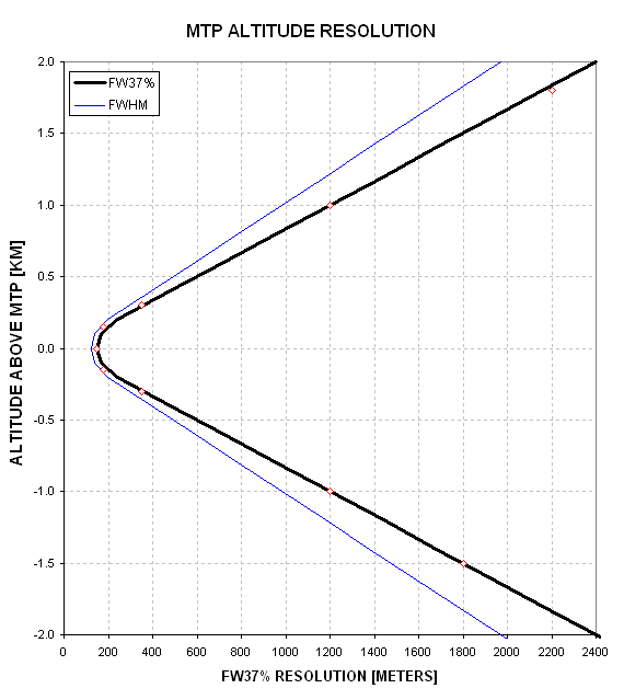
Figure 12.12. Averaging kernel width for retrieved air temperature versus altitude above MTP.
Check of Averaging Kernel Width Using Actual Retrieval Coefficients
The averaging kernel for a retrieved air temperature can be calculated by multiplying observable weighting functions by their corresponding retrieval coefficients.
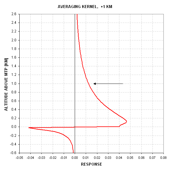
Figure 12.13. Altitude weighting function for retrieved temperature at +1 km above MTP.
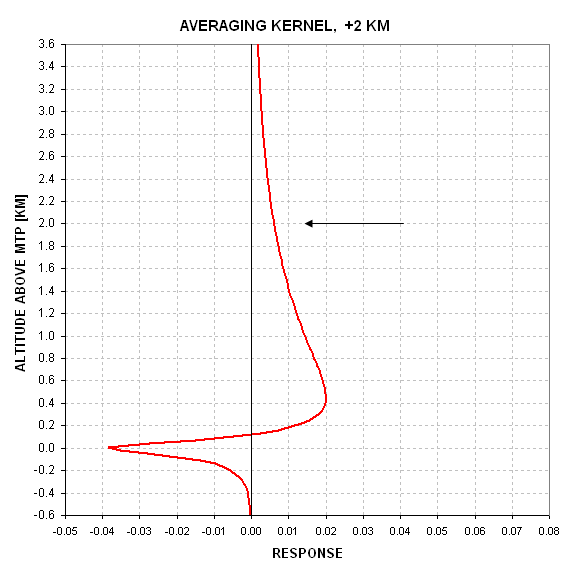
Figure 12.14. Altitude weighting function for retrieved temperature at +2 km above MTP.
In my opinion both of these averaging kernel shapes look bad! I think they're valid, since the kernel-weighted altitude agrees with the retrieved altitude. I suspect that the error matrix used in deriving the retrieval coefficients contained large enough a priori observable errors that the best solution was excessively "conservative."
Another thing to note here is that below-horizon observables were allowed in retrieving above horizon air temperatures. This might be unwise because in theory the below horizon don't contain any information about above horizon air temperature. The reason the below-horizon observables produce non-zero retrieval coefficients when they are included in the retrieval coefficient calculation is that temperatures below the horizon are correlated with temperatures above the horizon. A Backus-Gilbert solution would automatically assign zero values to the below-horizon observables, but the statistical retrieval procedure is less discriminating.
Performing statistical retrievals is an "art." Judgement has to be used, and there is no easy way to know what constitutes good judgement. One purpose for this web page is to promote humility for anyone employing statistical retrieval procedures. The ultimate measure of good performance is to compare retrieved temperature profiles with radiosonde profiles. But even when this is achieved there is no straight-forward ansewr to the question: "What's the MTP's altitude resolution?"
Go to next Chapter #13
Go to previous Chapter #11
Return to Introduction
____________________________________________________________________