This chapter is closely associated with Chapters 1 to 4. I deferred presenting the material until now because it is not necessary to understand antenna formulae in order to understand what the MTP observations mean. However, it may be necessary to trouble-shoot MTP performance in ways that involve the concepts antenna efficiency, beam efficiency and antenna pattern. These properties are related to each other in ways that allow two of them to predict the third. Read on.

In Chapter 1 a graph was given (Fig. 1) for the number of photons emitted (per second, per square micron, per unit wavelength) by a black-body surface at various temperatures. It was noted that the long wavelength regime has simple relationships, such that the flux of photons is proportional to temperature. This regime is referred to as the Rayleigh-Jeans distribution. Here is the formula for "black-body emittance" for this wavelength regime:



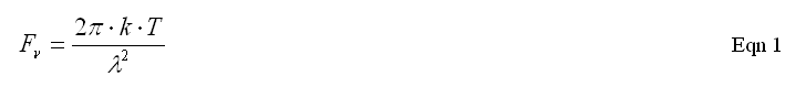
where Fv = power emitted by a unit area per unit frequency [watts per square meter per Hz frequency interval], k = Boltzmann constant (1.38 x 10^-23 [Joule/Kelvin]), T is Kelvin temperature, Lambda = wavelength [meters].

Consider a black-body surface at temperature T and distance R from an antenna having an antenna pattern f(theta, phi). The antenna pattern function is defined to be 1.0 at its direction of maximum reponse. We shall assume that the solid angle extent of the black-body is larger than the solid angle extent of antenna pattern (i.e., that antenna pattern is close enough to zero beyond the solid angle extent of the black-body that it can be neglected).



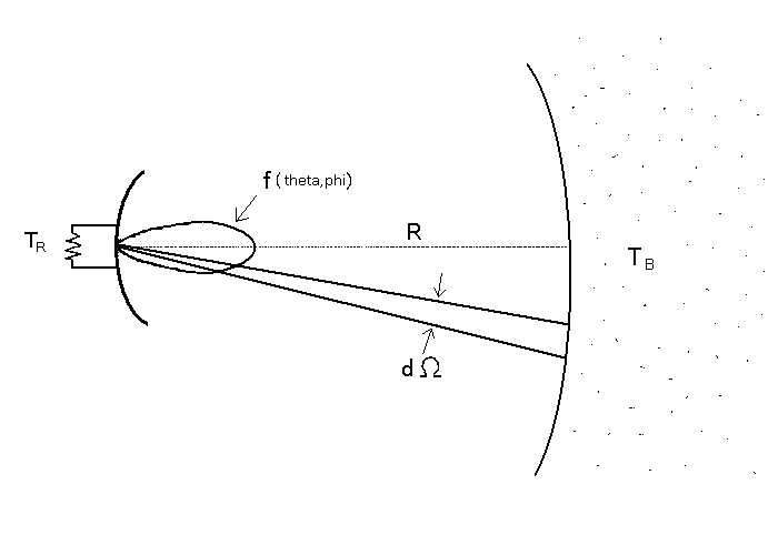
Figure 14.01. Antenna that receives radiation from a black-body at temperature T_B at distnace R from solid angle element dOmega with antenna pattern f(theta,phi) and delivers the received energy to a resister that warms to temperature T_R.

It is intuitively believeable, and physically true, that the resister will be heated to a temperature T_R equal to the temperature of the only part of the universe that it "knows about" (is in "contact with"), which is the black-body's temperature T_B. Another way of saying that is that the power received by the antenna and delivered to the resister is the same as the power produced by the resistor (for having a non-zero temperature) and delivered via the antenna back to the universe:

    P(out) = P(in), or

     

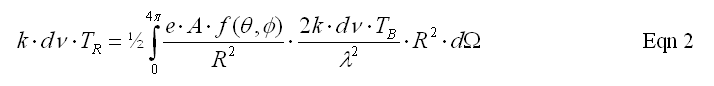
where dv = a frequency increment, e = aperture efficiency, A = physical area of antenna, Lambda = wavelength, R is the distance to the brack-body, dOmega = solid angle increment.

The left side of this equation is the power generated by a resistor at temperature T_R and the right side is the power received by the antenna and delivered to the resistor. The right side is an integral over all solid angles (2 pi) of the antenna pattern. Within the integral the first term is the solid angle of the apparent area of the antenna as seen by a radiating element of the black-body, which explains the presence of 1/R-squared. Within the integral the second term is the black-body emission of an increment of its surface area, which explains the presence of R-squared. (The 1/2 in front of the right side is due to receiving linearly polarized radiation from an unpolarized thermal source.)

This equation can be simplified: set T_R = T_B, which cancel each other, the two R² terms cancel, as do the two dv and k constants, and most of the remaining terms on the right side are constants that can be brought outside the integral. The result of simplifying is:

 

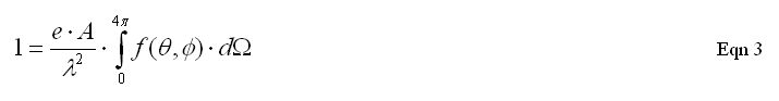
  where the integral can also be over whatever solid angle region corresponds to a non-zero antenna pattern.

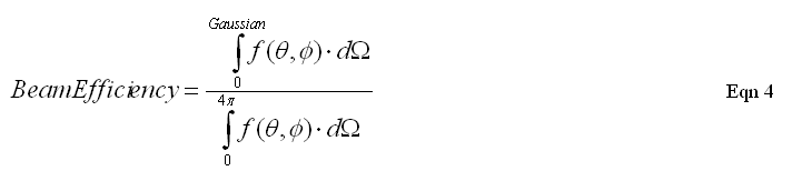
Consider representing the main beam of the antenna pattern using a Gaussian. Let's also define beam efficiency:



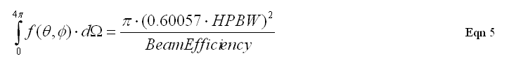
We know the integral of a Gaussian function, it's pi ( 0.60057 * HPBW )². (Note that HPBW must be expressed in radians.) Substituting this for the Gaussian integral in the above equation allows us to represent the second integral with simple parameters:

  

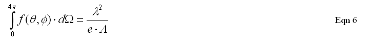
But we have another expression for the left-hand-side that comes from Eqn (3):

 

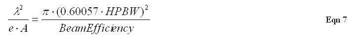
Combining Eqns (5) and (6) yields:



or



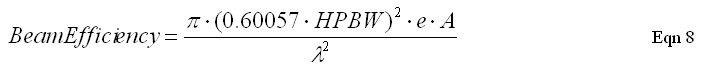
This expression for beam efficiency states that if we know aperture efficiency, e, and the Gaussian HPBW, we can calculate beam efficiency. When I first saw this derivation (in 1961; thanks, Fred Haddock) I almost fell out of my chair!

What an amazing relationship! I never imagined that from physics first principles it's possible to deduce beam efficiency from aperture efficiency, and visa versa. Measuring HPBW is easy, and aperture efficiency can be calculated from measured antenna temperature of a point source with known flux (I haven't given that in this tutorial, but it may turn up in a later chapter).

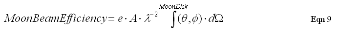
The term "beam efficiency" as defined above refers to the main beam, or an equivalent beam that is Gaussian and has a matching HPBW. There are special situations where we want to know the beam efficiency of a different solid angle. For example, the moon is circular with a diameter that for some radio telescopes is smaller than the antenna's HPBW, and for other radio telescopes it is larger than HPBW. When the beam is large compared with the moon we speak of "disk temperature" - which is the brightness temperature of a uniform disk with the same diameter as the object, that is uniform in brightness temperature, and that produces the measured antenna temperature. For the other case, common for large radio telescopes, the moon's disk is larger than the main beam and includes nearby sidelobes. For this case we want to define something I have referred to as "Moon Beam Efficiency" - or MBE. To calculate MBE from antenna temperature we need to know the antenna pattern out to the moon's edge (with the main beam centered on the moon's disk). Integrating the actual antenna pattern to the moon's edge produces a solid angle that can be substituted for the Gaussian solid angle in Eqn 7:



Here's a handy formula for Eqn (7) that employs common units:



For MBE this formula can be used if HPBW is adjusted upward slightly to account for the greater integral out to the moon's edge compared with the integral of a Gaussian that fits HPBW.
 
It should be noted that if you know your antenna pattern you can observe the moon and derive aperture efficiency. This assumes you know the moon's brightness temperature, which has been known to high accuracy for decades (thanks to the Apollo heat flow experiment and Steve Keihm's moon model analysis - with a little help from BLG). (Let's all urge Steve Keihm to produce a table or graph of model-based lunation-averaged moon center T_B, as well as lunation max-to-min range.)


Go to next Chapter #15
Go to previous Chapter #13
Return to Introduction