Calibrating Asteroid Observations
Bruce L. Gary, Last Updated 2015.01.25

This web page describes the way I calibrate observations of asteroids in a way that assures "CCD transformation" without using those horrendous CCD transformation equations.

Introduction

When combining observations from many observers in a study of variability it is important that each observer present magnitudes that conform to a standard band, such as V-band. The classical approach is to use "CCD transformation equations," which were developed many decades ago, before the advent of spreadsheets. It became clear to me ~ 15 years ago that the classical approach is inferior to a spreadsheet approach for at least 3 reasons: 1) CCD transformation equations are complicated, not intuitive and therefore prone to mistakes, 2) they don't allow for a non-linear fit that can sometimes be needed for transforming to a wide range of desired bands and 3) they're usually not graphically displayed, so identifying and removing "outlier" data (due to reference stars being variable, for example) is cumbersome even if attempted. If you're a glutton for punishment and still want to use CCD transformation equations, then be my guest; I derive them, and provide some cautionary tips for their use, at this web site: link.

The "modern" way for performing CCD transformations is described in the section "Sophisticated Processing" on this web page. A simpler method that can usually provide correct results is presented in the section "Simple Processing." I recommend trying the simple method, and if the combined light curve looks OK, stop there.

Simple Processing

For each FOV image set, calibrate (bias, dark and flat). Select a star for use as reference and another to serve as a check star. Use the V-mag for the reference star when doing the photometry. If both stars are constant (not variable with a periodicity comparable to the length of the FOV observation) then the check star should plot as non-variable and the asteroid's changes will be real. Copy the asteroid's V-mag vs. UT to somewhere and repeat for each FOV. Combining all FOV segments should produce a valid light curve (LC) with the rotation signal present.

A next step improvement on this procedure is to consider a few stars for use as reference and select the one with a B-V color most similar to the asteroid's color, which we think is B-V = 0.75. By doing this there should be smaller offsets between LC segments caused by not doing a CCD transformation.

If one (or more) LC segments persists in appearing to exhibit an offset with respect to the others, then this could be produced by the reference star used for that FOV being a long period variable, and it's V-mag at the time of observation is simply different from the APASS value. In that case, repeat that FOV's processing using a different reference star.

If the combined LC still exhibits a FOV offset pattern check with me for additional ideas.

Sophisticated Processing

For each FOV set of images do the following.  Calibrate (bias, dark & flat). Star align all images (I get better results using 1-star align). Print an inverted image for notation of the sequence of stars that will be used for reference. Add an artificial star to all images (download the MaxIm DL plug-in from here: AS). Invoke the MaxIm DL photometry tool. Identify the asteroid in an early image, check the "New Moving Object" box & click on the asteroid. Identify the asteroid in a late image, select "Mov1" and click the asteroid. Set the photometry signal aperture radius to ~ twice the FWHM in pixels, set the background annulus width to the largest possible value. Select "New Reference Star" and click the artificial star. Ignore entering a magnitude for it. Select "New Check Star" and click the first (unsaturated) star that you want to consider for use as a real reference star (in the spreadsheet phase of analysis). Note which star you selected on the printed image. Repeat for many more stars 9I like a couple dozen); they're all going to be labeled by MaxIm DL as "Check" when you record the CSV photometry file.  Note: For faint asteroids it really pays to employ "star subtraction" (usually doubles or triples SNR), as described here:  star subtraction. 

Using Excel, import the CSV file to a worksheet (I'll refer to "worksheets" as "pages" hereafter). If you're using a template spreadsheet especially created for this task (as I do), then you'll have a place to specify RA/DE, observatory latitude & longitude, and a calculation of air mass (based on JD). (Or, you can specify that air mass be included in the CSV file, if you're using MaxIm DL v6.x.)

On another page correct the mag's that you imported (which is usually referred to as "instrumental mag") for atmospheric extinction. This can be done by plotting total flux (of all stars) vs. air mass, etc. Or you can guess an extinction value and correct all instrumental mag's that way.

On another page enter BVg'r'i' magnitudes from C2A (or hand enter B & V mag's) for each of the reference star candidates (called "check star" when you were measuring them in MaxIm DL). There's a quick way to do this using the C2A "Export Objects" tool (under File menu) to create a CSV file which you can import to the spreadsheet, etc.  Create a "first offset parameter" that is applied to all mag's, and make a plot of these new mag's vs star color for all reference star candidates. The plot can look something like the following.

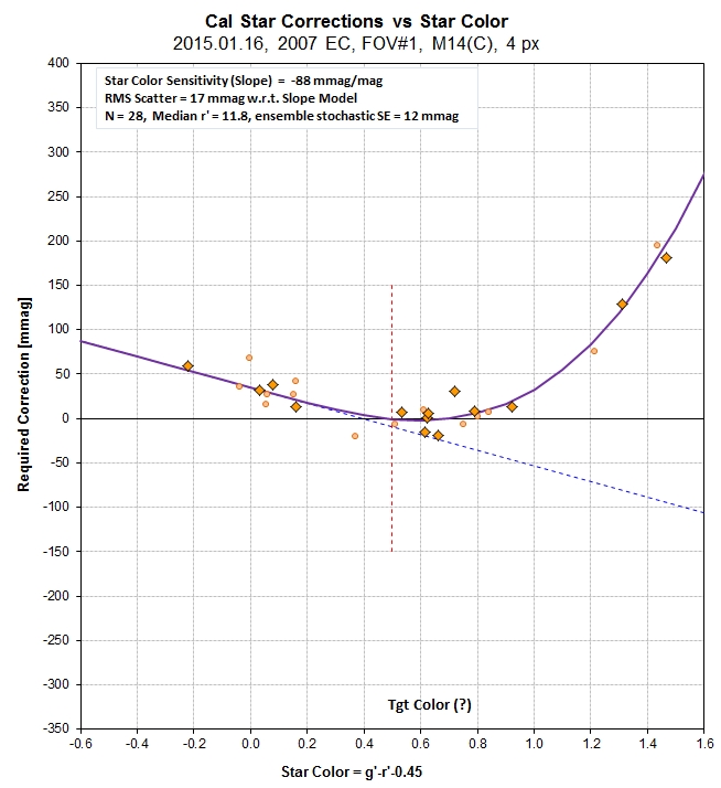
In the above graph notice that I defined star color to be g'-r'-0.45. Solar analog stars will have a star color of zero using this definition. Asteroids are typically redder than the sun, so I've set my target star color to be 0.50; that's where I want the model fit to be offset for "Required Correction" to be zero. The y-values are "candidate reference star r'-mag minus the "second offset parameter" (which is added to the "first offset parameter"). In this example a couple stars were identified to be outliers, so they were omitted from display. The RMS departure from this model fit is 12 mmag. If the APASS r' (and g' and i') mag's were perfect, with zero systematic error, we could state that the image set was now calibrated to an accuracy of 12 mamg divided by SQRT(N-2), where N is the number of stars used in the solution and 2 is the number of free parameter for the model. In reality, the APASS mag's probably have a systematic SE of ~ 101 mmag. Hence, the calibration using this method is closer to SQRT (12^2 + 10^2) = 16 mmag. That's acceptable for comparing one observer's asteroid magnitudes with another's. 

This site was opened 2015.01.25. Nothing on this web page is copyrighted.   BGary web sites