MESOSCALE FLUCTUATION AMPLITUDE STATISTICS
2000 January 10
Abstract
The mesoscale structure of isentrope vertical displacements have been studied using ER-2 and DC-8 Microwave Temperature Profile measurements of isentrope altitude cross-sections. Data from 94 flight segments have been fitted to an equation with 5 free parameters, yielding a solution that allows for the calculation of Mesoscale Fluctuation Amplitude, MFA, for a range of alitudes, latitudes, season and underlying topography. MFA is most strongly dependent upon an invented parameter that combines season with latitude. The greatest MFA values are found at polar latitudes, in winter, over mountainous terrain. MFA increases with altitude in approximate agreement with the expected "reciprocal square-root of air density" relation. It is suggested that the MFA equation be used 1) as an additional temperature fluctuation term for back trajectory calculations, and 2) in GCM calculations that require a method for modeling the altitude region where breaking gravity waves produce momentum flux that alters wind speed.Introduction
Microwave Temperature Profiler, MTP, isentrope altitude cross-sections, IACs, were used in 1987 to show that mountain waves penetrate the polar vortex tropopause and amplify with altitude in the lower stratosphere (Gary, 1989). In 1987 and 1989 MTP also measured the existence of an ever-present background of vertical displacements of isentrope surfaces having mesoscale spatial frequences. In polar regions, during winter, the amplitude of this structure was found to be greater for flight over land than flight over ocean (Gary, 1989; Bacmeister and Gary, 1990). This report describes a quantitative analysis of the amplitude of the mesoscale altitude deviations of isentrope surfaces from their smoother synoptic scale average. The measurement of mesoscale structure amplitude is based on Microwave Temperature Profiler data from selected ER-2 and DC-8 flights that were part of NASA-sponsored missions during the period 1989 to 1997.
A companion web page, Mesoscale Temperature Fluctuations, introduces the evidence for the mesoscale structure using airborne data. MTP IACs are shown to exhibit more structure than IACs based on synoptic scale "analyzed" temperature and wind fields. In the present analysis mesoscale structure is defined to be the difference between the measured structure and a 400-km double boxcar average (described below). Since air parcels traveling through isentrope structrues will undergo temperature fluctuations the structure is also referred to as Mesoscale Temperature Fluctuations, MTF. The amplitude of these vertical displacements can be quantified, using histograms, and I define a parameter called Mesoscale Fluctuation Amplitude, or MFA, to describe the histogram widths.
In preparing this report I have two user types in mind: 1) back trajectory users whoe want to estimate the effect of mesoscale dynamics upon the temperature history of air parcels, and 2) climate modelers who want to improve their calculation of horizontal momentum flux caused by the breakdown of gravity waves that have been amplified at high altitudes. It is important to assign realistic values of momentum flux to the wind field at the proper altitudes, and one of the present shortcomings of modeling studies is the lack of an adequate model for representing the magnitude of vertical displacements of gravity waves at altitudes below those where the wave breakdown occurs (Bacmeister et al, 1994).
Procedure
Mesoscale Fluctuation Amplitude, MFA, is defined to be the half-power full-width, HPFW, of the distribution of deviations of an isentrope surface from its synoptic scale average. I have arbitrarily chosen to use a synoptic scale averaging procedure that gives approximately the same result as low-pass spatial frequency filtering. My procedure is to calculate a 400-km wide boxcar average, which is subjected to a second 400-km boxcar averaging process. Histograms of deviations from this synoptic scale representation are then fitted to a Gaussian shape with manual adjustments of offset, height and width, using a spreadsheet application program. The resulting MFA results are entered into a data base where several independent variables are also entered: latitude, date, topography type and average altitude of the isentrope. Multiple regression analyses are then performed using various combinations of independent variables and MFA as the dependent variable.
Sample Flight
The following several figures are used to illustrate a typical analysis of a flight and the determination of MFA entries into a data base.
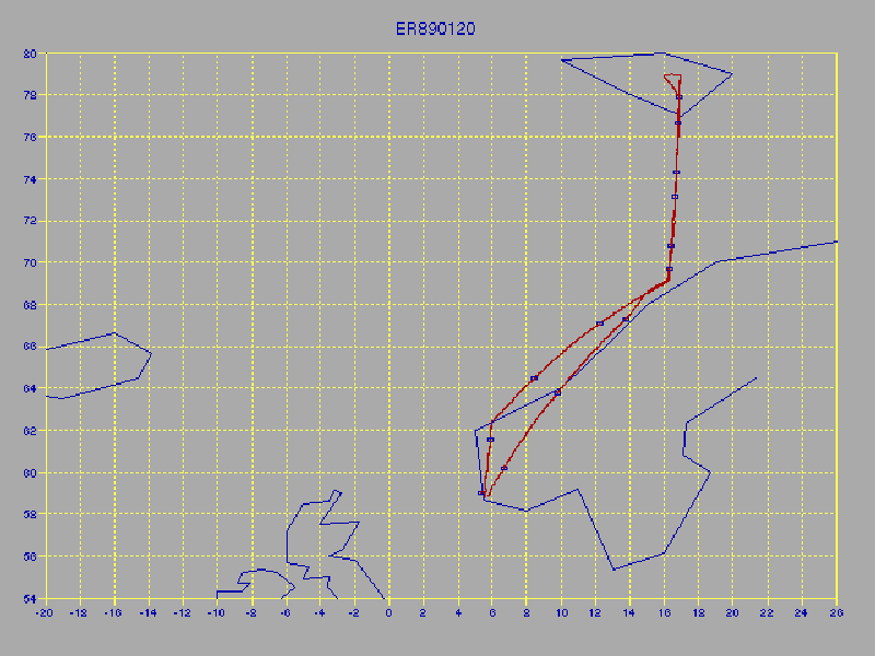
The figure below shows the flight track of a typical ER-2 flight used in the present analysis. It occurs under "polar winter" conditions, and is based in Stavanger, Norway. The flight date is January 20, 1989, which is represented as 890120 in the figure titles. Tick marks are shown at 2000 second intervals. The portion of flight within 100 km of the coast is categorized as "coastal mountain" and it is assigned a subjective topography roughness value. Since not all mountains have the same roughness, I have been guided by the following:
Land Type Topography Parameter
Ocean
0.0
Flat Land
0.4
Coast
0.6
Coastal Mtns
0.8 - 1.0
Continental Mtns 0.6 - 1.2
For the flight of 890120 the flight is divided into two types of flight segments, "coastal mountains" and "ocean," with topography roughness scores of 1.0 and 0.0, respectively.
Figure 1. Flight track for ER-2 flight of 1989.01.20, with markers at 2000 second (2 ks) intervals.
Next an "isentrope altitude cross-section," or IAC, is calculated from
the MTP data. The following figure illustrates this product, showing
the altitude of isentropes separated by 10 K of potential temperature.
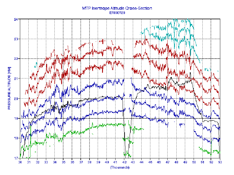
Figure 2. Isentrope Altitude Cross-section, showing the altitude of isentrope surfaces at 10 K intervals of potential temprature.
The IAC is used to choose a specific isentrope to represent flight segments.
In this example the 440 K and 460 K isentropes are used to represent the
pre-dip and post-dip flight segments. The isentrope altitudes for
these flight segments is shown in the following two figures.

Figure 3. Altitude of the 440 K isentrope for the first half of the 890120 flight.

Figure 4. Altitude of the 460 K isentrope for the second half of the 890120 flight.
The thick black trace in these two figures is my representation of a
synoptic scale fit to the MTP data. The departures of the red trace
from the black trace are used to create a histogram of "mesoscale only"
fluctuations. Since each of the previous figures shows data for both
"coastal mountains" and "ocean" categories, it was necessary to form the
histograms from carefully assigned segments of the two traces. Examples
of the two histograms are shown in the following two figures.
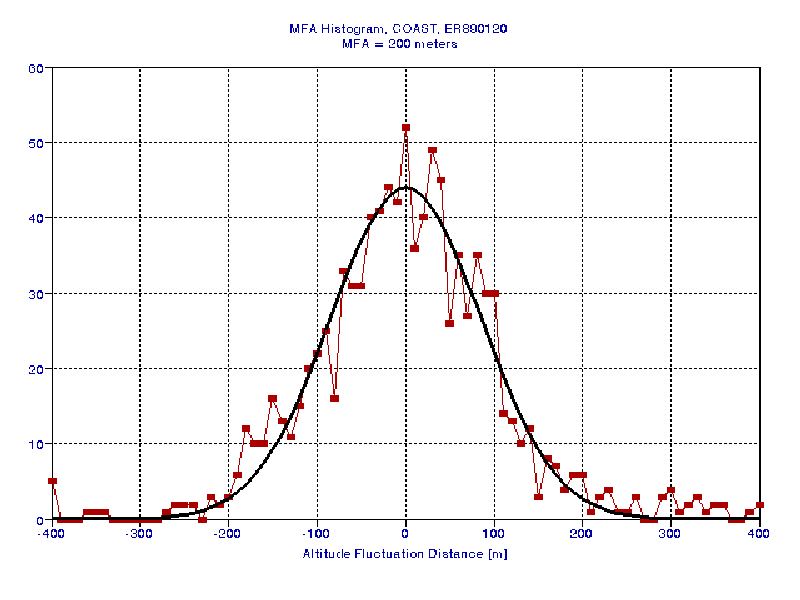
Figure 5. Histogram of all "coastal mountain" portions of the data shown in the previous two figures (for the 890120 flight).
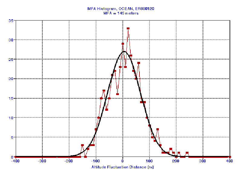
Figure 6. Histogram of all "ocean" portions of the data shown in the previous two figures (for the 890120 flight).
The foregoing analysis was performed for 49 ER-2 flights, comprising 73 flight segment topography assignments. The interval of flight dates extends from 881231 to 970925.
Summary of All ER-2 MFA Data
At the present time the data base for ER-2 flight data consists of 73 MFA values, corresponding to a range of latitdues, seasons and topographies. All isentrope altitudes are within the range 17 to 21 km, with an average altitude of 19.4 km. The next figure shows all 73 MFA values plotted versus latitude.

Figure 7. Plot of MFA values versus latitude. All seasons and topography types are included.
The general pattern in the above figure is that "MFA variability increases with latitude." When only "winter" and "summer" data are included, we get an insight into what causes the variability with latitude, as shown in the next figure.

Figure 8. "Winter only" and "summer only" MFA data are plotted versus latitude.
As the above figure shows there is a strong "seasonal effect" for MFA. It goes from "non-existent" in the tropics to "large" at the polar latitudes. I have employed a seasonal parameter that is sinusoidal with a winter maximum at January 22, which is one month after the winter solstice. It appears that the summer MFA values vary linearly with latitude, decreasing at the rate of 1 meter per degree of latitude. A fit to the summer data is shown in the next figure.

Figure 9. Empirical model fit to winter and summer only data (including all underlying terrains).
The thick red line is a linear fit to the "summer only" MFA data. The dashed blue line is a fit to the winter data, and it employs a quadratic dependence upon latitude. A multiple regression fit has been performed that uses the following independent variables: 1) latitude, topography, and season/latitude. The "season/latitude" paramter is simply: SeasonParameter * (Latitude/80)^2, where the SeasonParameter is sinusoidal ranging from 0.0 one month after summer solstice to 1.0 one month after winter solstice. Since a constant is involved, this least squares multiple regression fit has 4 independent variables. The equation for MFA is:
MFA = 134 - 1.6 * Lat + 202.5 * Seas*(Lat/80)^2 + 45.2 * Topo (Eqn 1)
where Lat is latitude [degrees]
Seas = (1 + sin (pi * (MN
- 10.7)/6))/2, and MN = Month number (1 = Jan, 2 = Feb, etc) + (Day of
Month) / 31
Topo = topography roughness
parameter, 0.0 = ocean, 0.4 = flat land, etc (see table, above)
The LS fit of this equation to the observed ER-2 MFA exhibits an r^2 = 0.63, and a residual MFA of 37 meters. The four constants in the above equation have values significantly different from zero, as the following table shows:
Const_1 = 134
Const_2 = 1.6 +/- 0.30
S/N = 5.2
Const_3 = 202.5 +/- 20
S/N = 10.1
Const_4 = 45.2 +/- 12
S/N = 3.7
From the S/N ratios (signal to noise ratio = ratio of parameter value to its uncertainty) the following conclusions can be made:
1) there definitely is a latitude effect,
2) there definitely is a seasonal effect
3) there definitely is a topography effect
The following figure compares predicted with observed MFA for the MTP/ER2 data.

Figure 10. Comparison of observed MFA with "predicted" MFA, using a 4-parameter model to fit dependencies on latitude, season and underlying topography.
The single "outlier" point in the above figure is associated with mountain waves extending along the coast of Norway (1989.01.19), and it should probably be omitted form an analysis that endeavors to represent the amplitude of the ever-present "background" of isentrope vertical displacements. The fitted line omits this datum.
Altitude Dependence of MFA
This section shows that MFA depends upon altitude. Since the foregoing analysis was with ER-2 cruise flight data, and is confined to a rather narrow altitude region (17 to 21 km), it should be possible to investigate the altitude dependence of MFA by plotting DC-8 MFA values on a graph having the ER-2 fitted line shown in the previous figure. Gravity wave theory predicts that wave amplitude should increase with altitude in accordance with the relation: A = A0 * (Rho0/Rhoi)^0.5, where A0 is an amplitude constant, Rho is air density, and Rho0 and Rhoi are air density at a standard level and an unspecified level. Since air temperature is approximately constant above the tropopause, air density will be approximately proportional to air pressure. This predicted dependence of wave amplitude versus altitude was observed by the ER-2 during encounters with mountain waves over Antarctica (Gary, 1989). What is true of mountain waves may not be true of an ever-present background of gravity waves, so it is necessary to verify the expected dependence of MFA on altitude.

Figure 11. Observed DC-8 MFA versus ER-2 predicted MFA, showing that at DC-8 altitudes (about 11.4 km) the observed MFA is smaller than at ER-2 altitudes (19.4 km). Green dotted line is based on the expected altitude exponent of 0.50, whereas the thick blue dashed line is based on a fitted value for the altitude exponent of 0.39.
The above figure shows that the MTP aboard the DC-8 observes smaller isentrope mesoscale fluctuation amplitudes than is predicted by the model that fits ER-2 data. In addition to the three effects noted above, by visual inspection of Fig. 11 it can also be stated that:
4) there is definitely an altitude effect.
The green dotted line is a prediction of DC-8 MFA based on the assumption that wave amplitude grows with altitude in proportion to the square-root of air pressure. To the extent that air density is proportional to air pressure, which it will be when air temperature is uniform between the DC-8 and ER-2 altitudes, the dotted green line corresponds to the predicted wave amplitude dependence upon altitude that holds for mountain waves. The thick blue dashed line is based on a fitted altitude exponent of 0.39, indicating that amplitude varies approximately as square-root of pressure, as predicted.
There are two "outliers" (upper-left) in Fig. 11. One (MFA = 210 meters, observed) is from a flight along the sub-tropical jet stream across the Pacific Ocean. The other (MFA = 260 meters, observed) contains mountain waves over the Rockies. These outliers suggest that data should be rejected from this type of analysis if they are associated with jet streams or mountain waves.

Figure 12. ALL data, ER-2 and DC-8, and a fit incorporating a free parameter for the altitude dependence of MFA. Three outlier data points have been deleted for this analysis.
Figure 12 contains data from both the ER-2 and DC-8. The mountain wave and jet stream outliers have been omitted. The fitted equation is:
MFA = (137 - 1.61 * Lat + 194 * Seas * (Lat/80)^2
+ 43.6 * Topo) * (58.85 / P [mb]) ^ 0.39 (Eqn
2)
+/- 0.30 +/- 18
+/- 10.4
+/- 0.10
where Seas and Topo are defined above, and P [mb] is the pressure of
the isentrope surface. Note the use of 0.39 for the pressure exponent.
The combined ER-2 and DC-8 data fit exhibits an R^2 = 0.61 and a residual
MFA of 32 meters. More data is needed to ascertain the statiscal
significance of the difference between the altitude exponent fitted solution
value of 0.39 and the predicted value of 0.50. Standard errors on
the estimate are shown below the 4 parameter fitted values. In every
case the SE is much smaller than the fitted value, with "signal to noise
ratios" (fitted value divided by SE) = 5.4, 10.6, 4.1 and 3.9.
[More DC-8 data will be added to this analysis, but the basic picture is unlikely to change.]
Specific Procedure for Simulating MFA
At this time Equation 2 is the best model representing MFA values over a wide altitude region, for all seasons, all latitudes and all topographies, and I recommend its use as a better alternative to a total disregard of the MFA effect. There are two ways to get a specific sequence for "vertical displacement versus horizontal distance," dZ(x), for adding to a back trajectory calculation of an isentrope surface's altitude. The hard way is to request a copy of a program that does this, which employs an algorithm described in Section 6 at Mesoscale Temperature Fluctuations. The easy way is to request a copy of a file "dZ(x)" from the author (BruceLGary@cox.net). The user may then modify the dZ column by a multiplication factor to convert it from having an MFA of 100 meters to the desired MFA. If a specific dZ(x) function is not required, but a probability density distribution for dZ is adequate, then this can be easily calculated from P(dZ) = EXP((-dZ/0.60*MFA)^2), which is normalized such that P(0) = 1, and MFA is first calculated from Eqn 2, above.
The following table of MFA values is based on the preceding analysis, and may be convenient for casual users wishing to estimate the possible importance of the MFA effect. To use the table, choose a latitude region (left-most column), choose a season (center two columns), and choose an underlying terrain (right-most column), and read from the body of the table an MFA. This MFA is what can be expected at ER-2 altitudes (19.4 km); for DC-8 altitudes, for example, multiply the MFA value by 0.61. For other altitudes, multiply the MFA value by (58.85 [mb] / P[mb]) ^ 0.39.
TABLE 1 - MFA for ER-2 Altitudes (19.4 km)
Multiply by 0.61 for DC-8 Altitudes (11.4 km)
| (Latitude Region) | WINTER | SUMMER | (Underlying Terrain) |
| POLAR | 239 meters
186 " |
68 meters
16 " |
Mountains
Ocean |
| MID-LATITUDE | 173 meters
121 " |
125 meters
72 " |
Mountains
Ocean |
| TROPICAL | 176 meters
124 " |
173 meters
120 " |
Mountains
Ocean |
Discussion
This is an "observational report" and not a study of dynamical meteorological processes at the mesoscale. Consequently, I am unqualified to speculate about the interesting dependence of MFA upon latitude, season or underlying terrain. However, I have never been shy about suggesting possible meteorological explanations for MTP observations, and being retired, I am even less shy about doing so now.
The fact that MFA is greater for "winter high latitudes" suggests to me that the independent variable I conjured up for the multiple regression analysis is merely a "proxy paramter" for wind speed. Support for this comes from the fact that I had to edit out high valued MFA outliers that corresponded to flight along jet streams (two occasions). The fact that clear air turbulence occurs preferentially during the winter season, which is conventionally attributed to the greater wind speeds in winter, is also supportive of this interpretation - since CAT occurs when KH waves are amplified by strong vertical wind shears in the presence of insufficient static stability (provided by the temperature field).
I am unable to suggest a credible explanation for the summertime latitude pattern (decreasing MFA with latitude). Help!
The dependence of MFA upon rough underlying terrain seems to require that the source for MFA is air moving over underlying terrain, causing vertical displacements that grow with altitude. This is supported by the near-absence of a correlation of MFA with underlying terrain during the polar summer (when winds are light).
Summary
For modelers wishing to assess the magnitude of mesoscale temperature fluctuations I recommend that Equation 2 (or Table 1) be used to calculate MFA, which then determines how to scale the sample sequence of dZ(x) available from the author, which can then be added to the synoptic scale isentrope altitude versus backtrajectory distance. For modelers wishing to calculate the altitude where wave breakdown occurs, I recommend that MFA be obtained using Equation 2 (or Tbable 1).
I further recommend that someone experienced in mesoscale dynamical meteorology take an interest in accounting for the MFA dependencies found in this study.
References
Bacmeister, J. T. and B. Gary, "ER-2 Mountain Wave Encounter Over Antarctica: Evidence for Blocking," Geophys. Res. Lett., 17, 81-84, 1990.
Bacmeister, J. T., P. A. Newman, B. L. Gary, K. R. Chan, "An Algorithm for Forecasting Wave-Related Turbulence in the Stratosphere," Weather and Forecasting, 9, 2, June 1994.
Gary, Bruce L., 1989, "Observational Results Using the Microwave Temperature Profiler During the Airborne Antarctic Ozone Experiment," J. Geophys. Res., 94, 112223-11231.
Related Links
Mesoscale Temperature Fluctuations Introduction to evidence for isentrope wrinkles (temperature non-uniformities) using airbore MTP data
Calculating "Colder Than Synoptic" Statistics Example of deriving MFA and "colder than synoptic" statistics
Clear Air Turbulence Overview of my views on CAT generation
Main Menu Meteorology and clear air turbulence web pages
Author: BruceLGary@cox.net
This site opened: December 13, 1999. Last Update: February 27, 2002