Introduction

As far as I know the airborne Microwave Temperature Profiler, MTP, is the only instrument capable of producing a topographic map of the altitude of an isentrope surface with mesoscale resolution.  Radiosondes have been used to produce synoptic scale versions.  Airborne in situ air temperature measurements could be use to create mesoscale versions, but they would require assumed knowledge of lapse rate near flight altitude throughout the mapped region.  Such an assumption would be especially risky in the presence of mountain waves, unless an MTP instrument were used to measure lapse rate.  But if MTP measurement are used, then it is trivial to convert the MTP temperature field to a potential temperature field, and thus derive the altitude of any isentrope surface near flight altitude.  To do this properly would require that flight legs be flown at approximately the same altitude in a raster-type pattern.  Since this is rarely done, the next best approach is to use MTP data for flights having a minimum of two ground tracks that are offset from each other.

The present web page is a report of results for two such flights, both of which contain mountain waves.  The first example is from an ER-2 flight in 1987, during the first NASA-sponsored "ozone hole" mission.  The sedcond example is from a DC-8 flight over Colorado during a NASA-sponsored mission to study contrails.  MTP data is available from ER-2 missions starting in 1986, from DC-8 missions starting in 1991, and a couple WB57 missions starting in 1998.  These archives may contain a half dozen additional cases for analysis if there is sufficient interest.  The two cases presented here provide good examples of the quality of MTP-based determinations of isentrope topographies in the presence of mountain waves.

MTP/ER2 Flight 1987.08.17

During the 1987 AAOE mission (Airborne Antarctic Ozone Experiment), the ER-2 flewover the Antarctic Peninsula many times while trying to penetrate the newly discovered "ozone hole."  The flight of 1987 August 17 affords an opportunity to explore the 2-dimensional shape of an isentrope surface due to the two north/south passes offset by about 40 km.  The two ground tracks occured close enough together in time that the isentrope surface did not change shape during the time interval separating the passes.

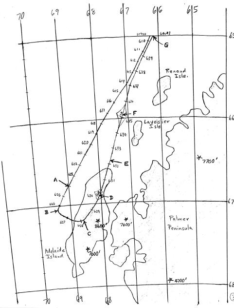
Figure 1.  Ground track of ER-2 during southern end turn-around.  North is at top, and longitudes and latitudes are labeled.

Locations "A" through "G" on this figure are used to show correspondences in the next figure.  "D" and "F" are times of ice cloud encounters.  The numbers beside the tick marks along the ground track are UTSEC in units of 100 seconds.  The "star" symbols denote mountain peaks, with altitudes [feet] noted.

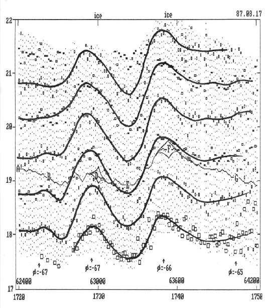
Figure 2.  Detailed isentrope altitude cross-section for the 30-minute flight portion centered on the mountain wave encounter.

Ice cloud encounters are shown at "D" and "F" in Fig. 2.  Hand-drawn lines show isentrope altitudes for 10 K theta (potential temperature) intervals.  Dots mark 2 K theta intervals.  At location "C" the ER-2 was flying parallel to the wind, which enables the isentropes in this region to be thought of as "streamlines" of air flow.  Isentropes in this region rise at the rate of about 1 km per 37 km of ground motion.  This corresponds to a real isentrope surface tilt of 1.5 degrees.  Since the wind was measured by the Meteorologigy Measurement System to be 40 [m/s], from azimuth 240-255, air parcels were rising at the rate of 1.08 [m/s], which corresponds to a cooling rate of 0.65 [K/mini, or 933 [K/day], assuming adiabatic processes.  The width of the upward sloping region is 44 km.  Note that the amplitude of the isentrope vertical displacements increases with altitude, as expected from theory (see AAOE Observational Results for data supporting this).

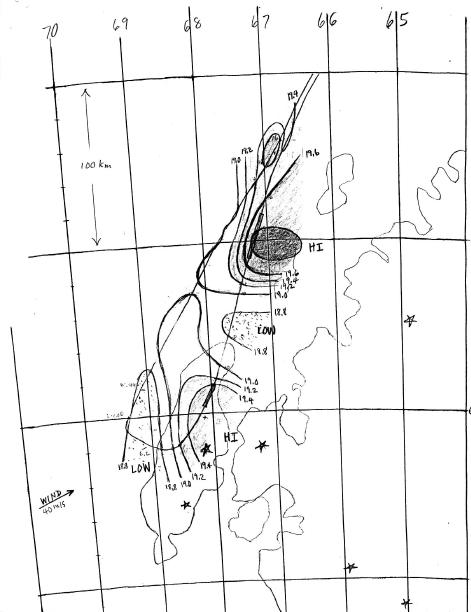
Figure 3.  Map of pressure altitude of the 420 K isentrope.

The southbound and northbound flight legs were offset about 40 km, which is a good value for properly sampling isentrope altitudes in the presence of mountain waves (which are assumed to be quasi-stationary).  The good agreement of isentrope altitudes at the north end of these tracks attests to the quasi-stationary character of the wave structure, since air parcels travelled about 100 km during the 40 minutes between ER-2 sampling times.  The iso-altitude contours are labeled with pressure altitude values.  The flight portions within ice clouds are marked by a widening of the flight track.  The southernmost high region was approached from a direction that is almost parallel to the wind.  This means we can interpret the first isentrope rise region in Fig. 2, locations "C" to "D", to be a good representation of what air parcels experienced during their encounter with this feature.

This is the first analysis of MTP data used to create a 2-D map of an isentrope surface.

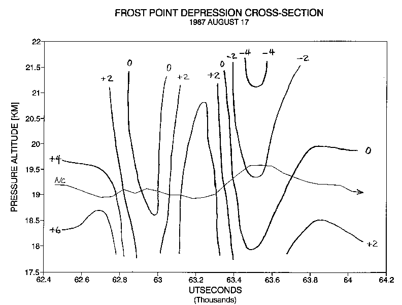
Figure 4.  Altitude/time cross-section of frost point depression, based on isentrope altitude cross-section (not shown here) and an assumed water vapor mixing ratio of 3.5 ppmv.

In this frost point depression cross-section there are two times when the frost point becomes negative, and they correspond almost exactly to the times that large aerosol particles were measured by the FSSP spectrometer (Guy Ferry, PI).  Particles in the 5 - 8 microns bin were measured, so they had to be ice crystals (not NAT particles).  [This figure doesn't directly relate to the goal of understanding the mopholgy of mountain wave isentrope surfaces, but is included here for investigators with other interests.]

MTP/DC8 Flight 1996.05.02

During the 1996 SUCCESS mission ((SUbsonic aircraft Contrail and Cloud Effects Special Study) the DC8 flew over the Rocky Mountains during an active mountain wave condition.  The following figures show the altitude of an isentrope surface.  The following figure is a ground track for a 4.5-hour portion of this flight.

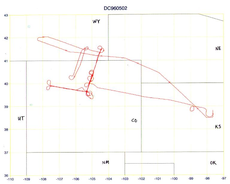
Figure 4.  Map of pressure altitude of the 420 K isentrope.

Notice the 4 passes over the same ground track in the southwest (middle Colorado).  The MTP data for isentrope altitudes is shown in the following figure.

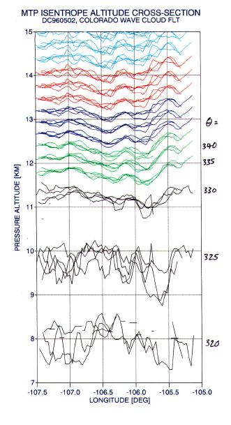
Figure 5.  Isentrope altitude cross-section for the 4 east/west flight segments in the southwest part of the region mapped in the previous figure.  The black traces are for the troposphere, and the colored traces are for the stratosphere.

The good agreement of the many east/west flight segments in the above figure shows that during a 1.5-hour period there is remarkable stability of the vertical distortions of the isentrope surfaces created by the mountain wave.  This provides confidence that 1) the MTP measurements of isentrope altitudes are "robust" (especially considering that one pair of crossings were at 11.91 km and the other pair at 11.29 km),  and 2) the other flight segments can also be combined to create a map of isentrope altitudes for a specific surface for the entire region sampled during 3 hours required to fly the criss-cross pattern in Fig. 4.

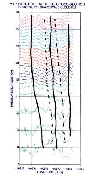
Figure 6.  Isentrope alttiude cross-section, showing "phase lines" tracing maximum vertical displacements.  Solid traces are upward, dashed traces are downward.

..

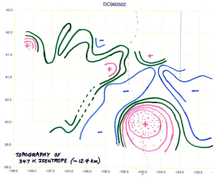
Figure 7.  Countours of altitude for one isentrope surface, covering the portion of the region in Fig.4 that was sampled by the DC-8.  The contour interval is 100 meters.  The lowest contour is 12.4 km (on the right side) and the highest is 12.9 km.  The Rocky Mountain continental divide is shown by a faint north/south dashed line that is underneath the highest vertical displacement, 13.0 km, located at the red "plus" symbol in the lower-right.

The figure, above, shows the altitude of one isentrope surface which appears to have been stable during the 4.5-hour interval required to sample it by the DC-8.  At the average altitude of 12.5 km the horizontal wind speed was 45 [m/s], from the west.  The slope on the upwind side of the big "+" feature has a rise to distance ratio of 1:51, corresponding to a slope of 1.1 degree.  Since the MTP measured slope involves some horizontal averaging, the rise ratio of 1:51 could be slightly conservative (meaning that slopes may be slightly greater, such as 1:40).  A 45 [m/s] horizontal wind therefore translates to a 0.9 [m/s] upward vertical velocity, or higher.  The north side of the big "+" feature has a rise ratio of 1:33, corresponding to a slope angle of 1.74 degree.   The Meteorology Measurement System, MMS, measured vertical velocities at the steepest slope region of +1.5 [m/s] during flight on the western edge of the big "+" feature.  This upslope vertical wind velocities are in approximate agreement.

For this Rocky Mountain case the upward sloping isentrope region is approximately 26 km wide (seen most clearly in Fig. 3).  The wave structure appears to be fixed with respect to the underlying mountains, with a persistence time of at least 1.5 hours, and probably 4.5 hours.  The vertical extent of the upslope wind is at least 3 km, and is probably much greater.  MTP remote sensing fundamental limitations cause the "measured" slope of an inclined isentrope surface to be underestimated by amounts that increase with the absolute value of the altitude difference between the isentrope surface and the MTP instrument.  Therefore, Fig. 3 does not show the expected increase of isentrope slope with altitude.  The fact that the slope value does not decrease noticeably with altitude implies that it actually increases with altitude.  A quantiative evaluation of this could be performed if there is sufficient interest.

Discussion and Summary

Isentrope surfaces are mapped for two mountain wave encounters, one at an altitude of 19 km and the other at 11.3 km.  For these events the upslope widths are approximately 44 km and 26 km, respectively, and the vertical air velocities are inferred to be +1.1 and +1.5 m/s.  For the second event the isentrope vertical displacement pattern appears to be "fixed" with respect to the underlying topography, and for the other case it was not possible to determine how fixed the pattern was.

Not all mountain waves can be counted upon to be "fixed" to the underlying topography for the same several hours found for the Rocky Mountain case.  For example, a 1987 September 22 mountain wave over the Antarctic Peninsula (see 870922 for a description of this "biggest" MTP mountain wave encounter) was found to change shape during the 1-hour interval separating the two flight segments through it.  Interestingly, this "same" mountain wave was present, at the same location, for three flight dates in a row, 870920, 870921 and 870922.  However, it appears to have been changing on a timescale of 1 hour on at least one date.

The MTP is a new tool for studying mountain wave dynamics on a mesoscale.  Someday I hope there will be an MTP investigation of mountain waves, with flight patterns designed specifically for measuring spatial, altitude and temporal features of the vertical displacement patterns.

This site opened:  February, 11, 2000.  Last Update: February 14, 2000