Introduction

The Microwave Temperature Profiler affords a unique opportunity to study the mesoscale structure of mountain waves.  It was during NASA's first airborne "ozone hole" mission to Punta Arenas, Chile, called AAOE (Airborne Antarctic Ozone Experiment), that the MTP/ER2 instrument measured the temperature field associated with a mountain wave that I have recently come to appreciate as the largest mountain wave an MTP instrument has ever encountered.  By some accident of fate, this was also the subject of the first computer-generated "isentrope altitude cross-section," or IAC using MTP data.  Since that day in 1987 I have produced hundreds of IACs from ER-2 and DC-8 NASA-sponsored flights, yet few come close to matching the 1987 Spetember 22 event for the wealth of detail that it provides.

Ground Track

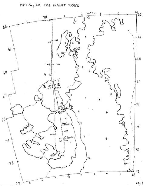
Figure 1.  Ground track for the flight of 1987.09.22, showing a portion of the Antarctic Peninsula.  Points "A" and "B" correspond to the highest and lowest displacements of isentrope surfaces near 20 km altitude during the southbound pass.  During the northbound (return) pass the locations "E" and "F" correspond to isentrope structures similar to "B" and "A".  At location "C" the ER-2 is descending through an adiabatic layer, from 15.8 to 16.8 km; at location "D" the ER-2 is at the same altitude but the lapse rate is normal at this location 150 km from point "C."  The numbers denote mountain peaks; for example, just left of location "B" is a 12, referring to 12,000-foot Mount Stephenson. The large island south of the mountain wave is Alexander Island.  The dashed lines trace the boundaries of permanent ice cover.

Isentrope Altitude Cross-Section

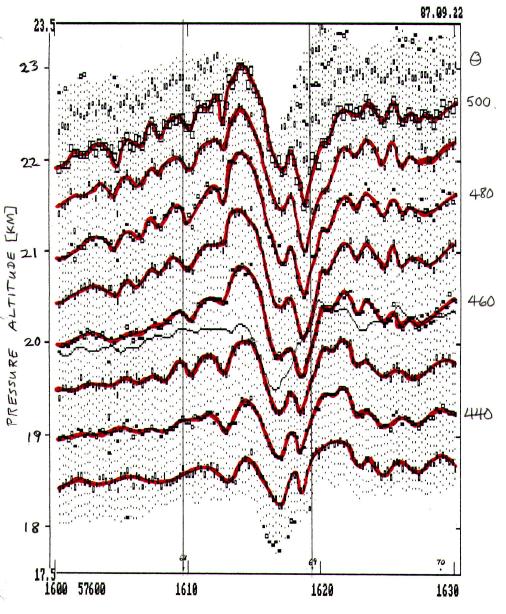
Figure 2.  Isentrope altitude cross-section for the first, southbound pass over Mount Stephenson. Imagine that we are looking eastward, in the direction of the wind, while the ER-2 is flying to the right, along the thin black trace, within a north/south plane defined by the page. The red traces are hand-drawn fits to isentrope altitudes. The two vertical lines are for latitudes 68 and 69 South.

The pilot's comment about this flight portion is that "these altitude excursions were imposed on me; I didn't initiate them."  There were no encounters of turbulence, and indeed there is no evidence of wave breakdown, so we are dealing with a smooth flow of air "into the page."  Mount Stephenson is located below the lowest altitude excursion, at 68.9 degrees South latitude.  The northernmost edge of Alexander Island is at 68.7 degrees South latitude, so the highest isentrope excursion is over a flat, possibly frozen ocean.

There are many noteworthy features in this IAC.  Let us assume that the "source" for this wave structure is Mount Stephenson, just 6 km upwind of the IAC plane and at 68.9 degrees South latitude.  First, there is a gradual rise of isentropes north of the "source" (i.e., prior to the main wave event).  From data not shown here, it was determined that the rise began at a latitude of 66 South, and this upward slope of "500 meters per 100 km span" is superimposed on a much gentler "synoptic scale" upward slope of "65 meters per 100 km span."  Thus, there are subtle distortions to the temperature field that extend 330 km north of the source, which corresponds to 330 km orthogonal to the wind direction.  The measured values given here are for the 480 K isentrope.

Second, at the highest altitudes a short wavelength structure is superimposed on the gradual rise.  Their wavelength in the plane of the IAC is 22 km.  The same waves are seen after the main encounter, south of the source.  The amplitudes of these waves appear to grow with altitude.

Third, the isentrope displacement field has a main spectral component with a wavelength of 45 at low altitudes and 57 km at the high altitudes, causing the lowest altitude for most isentropes to occur at 68.9 degrees South latitude (over Mount Stephenson) and the highest altitude to occur at 68.5 degrees South latitude.

Fourth, there appears to be a subtle "spreading out" of the "phase lines" (loci of maximum and minimum displacement) so that the location of maximum altitude is tilted to the left (in going upward), whereas the minimum altitude is tilted to the right (in going upward).

Fifth, the amplitude of long wavelength spatial components increase with altitude.  For example, the "highest to lowest" amplitude increases from 500 meters at an altitude of 18.5 km to an amplitude of 1540 km at an altitude of 22.3 km.

Sixth, there is a "beating effect" such that several waves are propagating upward in a way that changes the "shape" of the isentrope displacement versus latitude.  For example, whereas all isentropes are at their highest altitude at the same latitude (68.5 South), there are two latitudes that are "competing" for lowest altitude; the low altititude isentropes are lowest for the middle latitude contender (68.7 South) while the high altitude isentropes are lowest at the southern contender (68.95 South).

Seventh, at a latitude of 69 degrees South, at altitudes near flight level, the isentrope surfaces are sloped a very steep 2.7 degrees, for a rise to horizontal span ratio of 1:21, sustained over 15 km.  The wind direction was orthogonal to the flight direction, so the isentrope surfaces measured by MTP cannot be used as streamlines to infer air parcel ascent rates.  However, IF there were such steeply sloped isentropes in the east/west cross-section the horizontal wind speed of 35 [m/s], as measured by the MMS (Meteorology Measurement System) would translate to an upward ascent velocity of 1.7 [m/s].

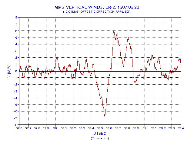
Figure 3.  Meteorology Measurement System, MMS, vertical winds throughout the time interval of the previous figure (16:00 to 16:30 UT).

This figure is derived from actual measurements of the vertical wind for the period graphed in Fig. 2.  It shows much higher vertical wind speeds, implying steeper isentrope slopes in the plane parallel to the wind (east/west), orthogonal to the flight direction.  A 6 [m/s] vertical velocity requires an isentrope slope of 9.9 degrees (given the horizontal wind speed of 35 [m/s]).  These vertical winds explain the ER_2 altitude chagnes; starting at 58500 seconds (16:15 UT) the ER-2 encounters a downward wind, which shifts abruptly to an upward wind at 58600 seconds (16:17 UT).  This figure also shows short wavelength oscillations prior to the main event, which exhibit a period of 84 seconds, or 18 km.  The isentropes prior to the main event have a spatial wavelength of 22 km, and the vertical winds have a spatial wavelength of 18 km.  It is not necessary that they correlate exactly, since the isentropes in the cross-section along the flight direction is a "snapshot" of isentrope location whereas the vertical winds are a snapshot of the vertical velocity of the isentropes, and the two parameters don't have to be "in phase."  If a hypothetical second ER-2 could have flown a few mintues behind the actual one, and if it had an MTP, then the vertical velocity of the isentropes could be inferred.  But lacking this information we cannot infer from an IAC taken at one time what the vertical velocities should be in a cross-section that is in a vertical plane orthogonal to the wind direction.

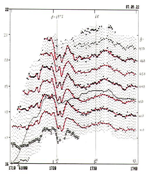
Figure 4.  IAC for the return flight leg through the same region of the main moutain wave event captured by the southbound flight.  Locations "E" and "F" in Fig. 1 correspond to the first minimum isentrope altitude and the following high altitude.

During the return (northbound leg) the ER-2 passes 7 km east of the southbound leg, and encounters the same mountain wave while flying at a lower altitude.  Due to the lower altitude the isentropes exhibit smaller vertical displacements.  At this location, or time, there seems to be a difference in structure, as described in the next section.

Changes Over Time
 

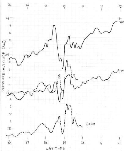
Figure 5.  Comparison of selected isentrope surfaces during the initial southbound flight leg (solid traces) and the return northbound flight leg (dashed traces).  The two IACs were measured about 1 hour apart.

The northbound isentrope structure correlates well with the southbound structure for latitudes 68.8 to 69.5 degrees South.  The correlation is poor at 68.7 degrees and southward.  Either there are strong east/west gradients, on a scale of 7 km (the flight track separation) or the isentropes are moving and evolving rapidly.  7 km corresponds to a distance equivalent to 0.06 degrees of latitude, and since the north/south IACs show only small altitude changes on this spatial scale I would prefer to believe that the isentropes were changing on a timescale of 1 hour.

Adiabatic Layer

Referring to Fig. 1, there is a notation of an adiabatic layer at location "C" that is encountered after the ER-2's turnaround and during a descent.  The measured dT/dz is -9.0 +/- 0.3 [K/km] throughout the altitude region 52,000 to 55,100 feet (15.85 to 16.8 km).  At this altitude and latitude, the adiabatic lapse rate is -9.7 [K/km] (I use the term "lapse rate" to mean dT/dz).  The measured lapse rate is very close to the adiabatic value.  Neighboring altitudes have a lapse rate of -2.0 [K/km].  This unusual layer was most likely produced by turbulence.  The turbulence, in turn, may have been produced by a mountain wave.  The adiabatic region is 30 km upwind of a 5000-foot mountain.  Perhaps the mountain distorted the upwind isentrope field sufficiently to create overturning, or, alternatively, the distortion produced KH instability where isentropes underwent vertical compression (bringing isotach and isentrope surfaces together, and lowering Richardson Number, Ri, to its unstable threshold value of 1/4).  Somehow, turbulence must have been triggered that ended in the production of an adiabatic layer.

When the ER-2 finished its "dip" descent, it ascended to resume a constant altitude return flight.  During the ascent, at the location marked "D" in Fig. 1, the ER-2 flew through the same altitude region that had earlier been found to be adiabatic.  However, at this same altitdue region, 150 km to the north, the lapse rate was "normal," varying between -2 and -3 [K/km].

Other details about this flight are available upon request.

Related links:

    Mountain Wave Isentrope Topography
 

This site opened:  February 13, 2000.  Last Update: February 14, 2000