This report presents results from the use of in situ "vertical wind shear" measurements for predicting CAT encounters. Vertical wind shear is combined with temperature lapse rate to derive Richardson Number versus time during flight.  A 3.6-hour segment of flight 88.12.29 (over the US) shows a "close to expected" pattern of Reciprocal Richardson Number, RRi, versus time in relation to a light CAT encounter.  After analysis of the first half of this data, four predictions were made of the RRi pattern for the second half.  Three out of four of these predictions are supported by the subsequent data. This is an exciting result, and provides support to a theory for CAT generation, also summarized in this report.

Introduction

I have proposed that vertical wind shear, VWS, can be derived from in situ measurements of the horizontal wind vector, air temperature and pressure, and MTP-derived air temperature lapse rate.  From these it is possible to determine Richardson Number, which is generally recognized as having CAT encounter predictive capability. To my knowledge, the data presented here is the first airborne test of this hypothesis.

Air temperature and pressure data were obtained from the Meteorology Measuring System, or MMS (Chan, et al, 1989), which is mounted on one of NASA's ER-2 aircraft based at the Ames Research Center. The present analysis is restricted to a 3.6-hour segment from the 88.12.29 ferry flight from Ames Research Center to Wallops Island, during which there is an encounter with light CAT.

An earlier version of this report described the first 1.4 hours of data, and based on these results predictions were made concerning the following 2.2 hours of data. This report retains much of the text of the first report (including the descriptions of the rationale for the data analysis employed), repeats the predictions contained in the first report, and presents the results of evaluating the predictions.

Model for What to Expect

I invite the reader to imagine that the stratosphere consists of a stack of air masses, overlying each other, with shallow transition layers between them. Each air mass moves in a distinct horizontal direction, governed by its history. Vertical wind shear, naturally, is concentrated in the transition layers. Temperature contrasts are also concentrated in the transition layers, and these layers are often "inversion layers."

The presence of the transition layers can be inferred from vertical profiles of RRi, the reciprocal of Richardson Number. RRi can be thought of as the ratio between overturning forces to stabilizing forces. The transitions are marked by enhanced values of RRi. Since air masses can have a component of vertical motion, the interfaces are not always horizontal. Flight at a constant altitude may sometimes intersect the transitions layers.

CAT is generated when RRi exceeds 4, and it persists until RRi becomes less than 1. It is still open for speculation how far below 1 RRi will be driven by the homogenizing action of CAT.  In non-CAT regions RRi has values of 0.1, typically. Since air for which RRi > 4 will produce CAT throughout neighboring regions meeting the criterion of RRi > 1, there is always the possibility of CAT when RRi > 1. Further, since CAT is felt at layers that border the altitude regime where it is generated (albeit at a lower severity level), it is important to keep in mind that CAT can even be encountered when RRi < 1.  If RRi varies gradually with altitude, then larger RRi values can be expected to be associated with greater probabilities of CAT, even when RRi < 1. Thus, the probability of CAT at given intensity levels can be expected to increase in going from RRi = "typical" to RRi = "borderline," where typical  0.1 and borderline  1.

It is also important to keep in mind that CAT reduces RRi, bringing it closer to "typical" values with a timescale that may be short compared to the life of the CAT.  In other words, CAT may quickly "wash out" the high RRi values that generated it, then linger at ever-decreasing severity, during which the energy in the vortices cascade to smaller and smaller scales (eventually  becoming "thermalized").  Hence, if CAT produces RRi values that are < 1, yet are still > 0.1 (the normal background level), these regions should have a finite probability of being turbulent due to the difference in timescales for RRi destruction and CAT dissipation.  The sum of these several arguments suggests that RRi values below 1 may not be as  "innocent'' as first-order Kelvin-Helmholtz wave theory and Richardson Number stability theory would suggest.

Figure 1.  Sequence of RRi(x) for an interface layer between two air masses, one overriding the other, at different stages of CAT generation.

Figure 1 depicts traces of RRi versus horizontal location within an imagined inversion layer that separates air masses, one overridding the other, at different times during the generation of CAT.  It can be imagined to be a horizontal transition layer that is close to instability for only the middle portion, or it can be imagined to be a produced within a transition layer that is slightly inclined to the horizontal, which is close to the threshold for becoming unstable throughout a much larger horizontal extent than is shown. The following arguments will be valid for either imagined geometry.  Let's imagine that the RRi traces are produced by a specially instrumented aircraft flying through the interface layer at different times.

Panel la shows RRi versus flight time, and the central part of this plot exhibits RRi above normal and slightly exceeding RRi = 4 at the center. We are to imagine that CAT has not yet been generated because the instability criterion has only recently been reached.

Figure lb shows what might be observed on a later flight through the same region, after an outbreak of CAT occurred where RRi had exceeded 4 for a sufficient time.

Fig. 1c is for an even later flight pass, after several patches of CAT have occurred. At this time the CAT from these outbreaks is still dissipating, which I assume takes longer than the initial homogenizing of the transition layer (and reduction of RRi).  Thus, CAT may still be encountered where RRi has been reduced, but it is not encountered where RRi is still high (or where RRi has never been high).

In Fig. 1d all the high RRi regions have produced CAT, and the transition layer has "exhausted itself" of CAT-producing vertical wind shear.  All RRi values are < 1, and perhaps << 1.  We must be prepared, however, to expect residual CAT (at some intensity level) to exist throughout the middle region of Fig. 1d.  If the remnant RRi values distinguish themselves from the normal background levels, then the "intermediate" values for RRi might be associated with light CAT.

Note that there is a negative correlation of CAT with RRi within the region of initially high RRi. The distance scale of the initially high RRi (the field of CAT patches) is typically 500 to 1000 km, whereas the distance scale for the individual CAT patches is 20 to 50 km. Therefore, with this model we predict a negative correlation of CAT with RRi for distance scales of less than 100 km, and positive correlations for distance scales exceeding 100 km.

Kelvin-Helmholtz wave amplitude is theorized to grow unchecked, and trigger CAT, provided RRi > 4 for a sufficient length of time.  CAT sustains itself (ie, continues to extract energy from the horizontal wind field, and eventually thermalize that energy) until RRi < 1. When KH waves overturn they homogenize the CAT layer by stochastically exchanging air parcels. This process leads to a reduction of the vertical wind shear to very low values, and also produces a fairly uniform potential temperature field (and thereby completely destroying any pre-existing inversion layer). Thus, I will allow for the possibility that CAT converts air from RRi > 4 to RRi < 1. Perhaps RRi is reduced to values much lower than 1, such as 0.1.

It should be kept in mind that RRi and CAT have 3-D distributions.  The sequence of CAT formation and spreading can be expected to have distinct patterns in the vertical. For example, CAT may start at a middle altitude (where RRi = maximum, presumably) and spread vertically in both directions toward the upper and lower edges of the transition layer. Another complication to keep in mind is that in the real world flight paths can course through these distributions at odd angles and in a curved manner. This complication wiil especially have to be dealt with when designing CAT warning algorithms for ascents and descents.

VWS Algorithm

My proposed method for determining VWS requires in situ measurements of the U and V wind components (the EW and NS components of the horizontal wind vector), air temperature and pressure, and MTP-derived air temperature lapse rate, which I define as dT/dz.  Air temperature and pressure are combined to form the much more useful atmospheric parameter "potential temperature," theta, defmed by:

    Theta = T[K] * (100/BP[mb])^0.286

Surfaces of equal theta are called "isentropes," and since theta is a property of the air that does not change with an air parcel's (adiabatic) altitude excursions isentropes can usually be thought of as streamlines for air movement.

The crucial insights leading to the realization that VWS can be derived with existing sensors, and which is used in the present analysis, is summarized by the following two facts:
 

1) dU/dtheta and dV/dtheta can be measured using in situ measurements of U and V while theta is also measured; this is done by creating scatter plots of U and V versus theta during altitude excursions of either the aircraft or isentrope surfaces, and

2) these theta-derivatives can be converted to altitude derivatives by simply multiplying by dtheta/dz, which can be calculated from knowledge of air pressure and dT/dz (measured by the MTP instrument).

These two steps allow calculation of  dU/dtheta and dV/dtheta which can be orthogonally added to produce the vector value of horizontal wind shear, VWS, which is the crucial parameter needed for calculating Richardson Number. A more compact equation for Richardson Number  (and its reciprocal) is derived in the attached Appendix, and it is this equation which has been used in the present analysis.

I think it will be instructive for the reader to follow derivations of more familiar atmospheric properties, such as VWS, even though VWS is not explicitly calculated in my preferred procedure for deriving Ri. The next several paragraphs are presented with this preference in mind.

In the present analysis it was found that 30-second chunks of MMS data were close to the optimal length for the purpose of performing least squares regression analyses in which the U and V wind components are chosen, in turn, to be the dependent variable, and time and 0 are used simultaneously as independent variables.  The regression analysis produces solutions for the gradient of the wind components with time, dU/dt and dV/dt, the gradients of the wind components with theta, dU/dtheta and dV/dtheta, and the RMS fit before and after the fitting analysis, RMSo and RMSf.

Three-point weighted averages of the partial derivatives of U and V with theta were found to be less affected by horizontal wind gradients, provided a proper weighting equation is used.   The weighting is performed on the U and V gradients separately, using the following equation:

Weight = 1/{(1 + (HG/5.6)^2 + (RMSf/35)^2}

where HG = dU/dt or dV/dt .  The weighted-average dU/dtheta and dV/dtheta  can be converted directly to dU/dz and dV/dz by multiplying by dtheta/dz.  If this were done the orthogonal sum of the resultant derivatives of U and V with z would correspond to the desired VWS.

Another (equivalent) path is also possible, which preserves like-observables for as long as possible in the derivation (and corresponds with the derivation in the Appendix).  The orthogonal sum of the two theta-derivatives of U and V can be formed, called "VWStheta" [m/s per thetaK]:

    VWS0 = {(dU/dtheta)^2 + (dV/dtheta)^2}^1/2

By multiplying "VWS0" by "dtheta/dz"  we obtain VWS [m/s per km], the vertical gradient of horizontal wind in terms of altitude, z (instead of theta).   dtheta/dz  [thetaK/km] is calculated from MTPderived lapse rate, dT/dz  [K/km], and MMSmeasured air pressure, BP [mb], according to the relation:

     dtheta/dz  = (dT/dz + 10) * (1000/BP)^0.286

By combining these equations we obtain a relation for VWS [m/s per km]:

    VWS = VWStheta * dtheta /dz

where the two terms on the right are defined above.

Normally Ri is stated in terms of the parameters just described:

    Ri = g/theta * (dtheta/dz)/VWS^2

However, in the Appendix an expression is derived for Reciprocal Richardson Number, RRi, which is easily converted to Ri by taking the reciprocal.  The expression in the Appendix is esthetically better because it contains quantities that are "closer" to the observed quantities, so it is easier to implement.  The expression is:

    RRi = (theta/9800) * (dT/dz + 10) * (1000/BP)^0.286 * {(dU/dtheta )^2 + (dV/dtheta )^2}

where theta has units [K], dT/dz has units [K/km], and dU/dtheta and dV/dtheta have units [m/s per K].  Reciprocal Richardson Number (= 1/Ri) is better "behaved" than Ri when temporal averaging is performed, which is the reason RRi is used more extensively in the present analysis.

CAT intensity, CATI, was calculated from the MMS measurement of "vertical acceleration."  The maximum 1-sec peak-to-peak spread (of 5 Hz data) during 5-second intervals was chosen to represent CATI.  This definition was found to have desirable properties (ie, it was not influenced by wave motions having periods longer than a few seconds, yet it "captured" short-term CAT excursions).

Results for 3.6-hour Data Segment

Figure 2 shows detailed tracks of both horizontal components of the wind field as a function of theta.

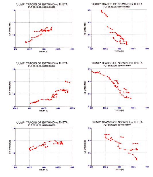
Figure 2.  Three 20-second sets of wind versus theta tracks, showing "jump" tracks.  Left column is for the U, or EW-component of wind, while the right column is for the V, or NS-component of wind.  Note the pattern of lower-left to upper-right for the left column, and upper-left to lower-right for the right column.  The U-component of VWS is poistive, while the V-component of VWS is negative.  The total VWS, being the orthogonal sum of the U- and V-components, is approximately 30 [m/s per km] during this period.

The left three columns show that for three successive 20-second intervals the U component increases with 0, with a slope of about +1.0 [rn/s per 0 K]. The V component decreases with theta with a slope of -2.0 [m/s per  K].  The gradient of the wind vector shears at the rate of:

    VWS0 = (1.0^2 +2.0^2) =  2.2 [m/s per  K].

During the first 1.4-hour flight segment dT/dz averages -1.5 [K/km] (varying within the range -2.5 to +0.3 [K/km]), theta  = 468 K and BP averages 56 [mb].  For these conditions:

    RRi = 0.93 * {(dU/dtheta )^2 + (dV/dtheta )^2}

when the  theta wind gradient is in units [m/s per thetaK].  For a  theta wind gradient of 2.2 [m/s per  K] we calculate that RRi = 2.0, or Ri = 1/2.  This air is close to the critical threshold for Kelvin-Helmholtz instability, considering that RRi typically  has values < 0.1 (ie, Ri is typically > 10).

Figure 3.  CAT intensity, based on vertical accelerometer data.

Figure 3 is a plot of CAT intensity versus time during the 3.6-hour flight segment that has been analyzed here.  The flight track extends from Western Utah (at 60 ksec) to Western Kansas (at 65 ksec) to West Virginia (at 73 ksec).  (I will use the term "ksec" to represent the time coordinate "UT seconds.")  The brief patch of CAT at 63.0 ksec is over Pikes Peak, and might be mountain wave CAT.  The other CAT patches are not associated with mountains.

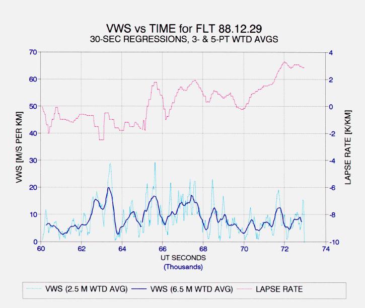
Figure 4.  Plot of dT/dz, from MTP instrument, and RRi, using algorithm described in this report.  The light blue trace is a 2.5-minute weighted, running average of the 3-second individual RRi values, and the dark blue trace is a 6.5-minute weighted, running average of RRi.

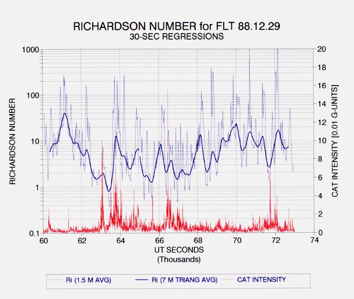
Figure 5.  Plot showing Richardson Number versus time the light CAT encounter.

In Fig. 5 Ri is seen dipping below 2 for the first time at 62.5 ksec, and 8 minutes later, at 63.0 ksec, light CAT is encountered.  There is a pattern of low Ri from  62.5 to 69.0 ksec, where Ri is generally < 5.  Outside this region Ri is typically ~10.  The thick trace for Ri is actually the reciprocal of running averages of RRi (which accounts for the trace tending to follow the lower region of Ri excursions instead of the upper region).

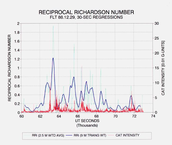
Figure 6.  Reciprocal Richardson Number versus time, showing the rise of RRi BEFORE and AFTER the light CAT encounter at 64 ks.

Figure 6 plots RRi and CAT intensity versus time for the same flight segment.  The 2.5-minute averaged RRi trace reaches a maximum of 1.9 at 63.4 ksec.  (The unaveraged data shows a maximum of 2.2 at this time, consistent with the data of Fig. 2, which was for this time.)  Immediately after the peak in RRi one of the main CAT events begin. There is a negative correlation of CAT with RRi within the early part of the "CAT containing region."  CAT patches extend from 63.0 to 67.0 ksec (referring to Fig.3).  The pattern of high RRi extends from 62.5 to 69.0 ksec, a slightly larger region.

It is possible to imagine that before the outbreak of CAT patches the RRi trace rose from ~ 0.1 to values > 1, and perhaps as high as 4 throughout the "CAT containing region."  As each CAT patch occurred it quickly reduced RRi to low values, and was left surrounded (horizontally) by high RRi regions.  We can imagine that the edges of the "CAT containing region" are the last to generate CAT; ie, that CAT patches occur first near the center of the high RRi region, and "randomly" occur at locations that move toward the outer edge of the high RRi region.  At some stage in this process there may exist an outer ring of high RRi, inside of which RRi is low but turbulent (with decaying CAT).  This would provide an ideal geometry for predicting CAT encounters.

Predictions Based on First 1.4 Hours of Data

This remainder of this section, which I have italicized, was written when only the first 1.4 hours of data had been analyzed (up to 65.0 ksec).  It is preserved here, unaltered, as a way of illustrating the reasoning which motivates my conception of CAT generation, and which may be useful in guiding the development of CAT warnings and avoidance strategies.

"The pattern of RRi and CAT versus time presented here is consistent with the model for CAT generation described in this report. Predictions can be made, using the model, for what will be observed for the next 83-minute data segment when it is reduced.  I predict the following things:

     1) The negative correlation between CAT and RRi will persist until the other edge of the CAT containing patch is reached (at 68.0 ksec),

     2) RRi will vary within the range 0.05 to 1 from 62.5 to approximately 68.0 ksec (I'm assuming that RRi has symmetry with respect to the region containing CAT),

     3) RRi will be high from 67.5 to 68.0 ksec (which will be the counterpart to the region 62.5 to 63.0 ksec,  assuming symmetry, again), and

     4) Beyond 68.0 ksec RRi will decrease to < 0.05 and stay low.

This analysis will be conducted immediately after submitting this report, and a follow-up report will be issued when the predictions have been tested."

How the Predictions Fared

The italicized section, above, is taken from an earlier report, when the laborious hand-analysis had progressed only as far as 65 ks.  This section follows-up on the predictions of the earlier report.

Prediction #1 is not supported; there is no correlation between CAT intensity and RRi during the part of "CAT containing region" after 65.0 ksec.

Prediction #2 is supported.  The values for RRi do vary within the range 0.05 to 1 for the part of the "CAT containing region" after 65.0 ksec.

Prediction #3 is supported, though weakly.  There is a collar of relatively high RRi after the last CAT patch.  The last CAT patch ends at 66.6 ksec and RRi is high from that time to 67.6 ksec. Thus, there is a 1.0 ksec collar of high RRi beyond the last CAT patch. The high RRi collar before the first CAT patch is 0.6 ksec wide.  Both collars have RRi values of about 0.6, though the first collar contains higher values for brief periods.

Prediction #4 is partially supported.  RRi values are low most of the time after passing beyond the last collar.  The main exception to this is the "second collar" of moderately high RRi from 68.3 to 69.0 ksec.  A brief area of high RRi occurs at 71.6 ksec (and it appears to be associated with very light CAT).

The RRi criterion for distinguishing between CAT patch association and no association seems to be 0.2 (ie, Ri = 5).  Within the "CAT containing region," which I define as including the "collar" regions (ie, from 62.5 to 67.6 ksec), RRi exceeds the proposed RRi criterion 85% of the time.  Outside the "CAT containing region" RRi exceeds the RRi criterion only 16% of the time.

[Note, added 1999, September 19:  This CAT encounter was "light" and is not an ideal case for evaluating the RRi collar theory, although the RRi collar theory is supported by this case.  A better CAT encounter exists for illustrating the merits of using RRi(t) to warn of CAT, and will be presented in a future web page.  The purpose of reproducing this report is record a description of a procedure, or algorithm, for calculating RRi from INS-winds and MTP lapse rates.]

Commentary

Measuring "vertical wind shear" in this manner, and thereby inferring Ri and RRi, has never been tried before (as far as the author knows).  It is a new tool that should, on theoretical grounds, have relevance to CAT prediction.  There may be errors in estimating VWS this way, leading to VWS underestimates (or possibly over-estimates).  It is nearly impossible to verify that the VWS values are correct - short of flying two aircraft in formation, one slightly above the other.  Comparing the new VWS measurements with CAT encounters provides an indirect way of verifying that the values are approximately correct.  The results, so far, are extremely encouraging.  If the "collar pattern" of VWS-based RRi continues to correlate with CAT in a "useful" way, the question of whether the new VWS measurements are accurate becomes moot (for the user interested in predicting and avoiding CAT). The motto "If it works, use it!" would then apply.

A larger community exists, however, who would like to know if such a simple method for inferring VWS actually works.  Meteorology researchers, such as those studying vertical mixing processes, would like to know if VWS can actually be measured without adding instrumentation to their aircraft.  These potential users of the in situ method for inferring VWS deserve to know more about how well the method works.

The data reported here seems to imply that VWS is being under-estimated. The theoretical model for CAT generation which I described calls for RRi values of 1 to 4 within the "CAT containing region."  Instead, values of 0.5 to 1 were found.  This suggests that VWS is being underestimated by approximately a factor of 2, and perhaps as much as a factor of 4!  I see two possible ways to account for this apparent discrepancy.

First, there would be no discrepancy if the flight data for this region of CAT patches is interpreted as being on the lower or upper edge of an unstable region, and the CAT that was experienced was being generated at a different altitude. This interpretation might account for the very light nature of the CAT.

Second, VWS is under-estimated using this technique because air parcels of size 2 km or so "take on" part of the horizontal velocity of the air into which they make vertical excursions, causing their horizontal velocity vector to oscillate as their altitude oscillates. For example, if an air parcel's size and oscillation period are such that its instantaneous velocity is exactly intermediate between its time-average velocity and the velocity of the surroundings,  then VWS would be underestimated by a factor of 2.

This last interpretation of the new method for estimating VWS underscores the importance of understanding "how does it work?"  This matter needs to be addressed by a mesoscale meteorologist sometime.

I have become very much aware, during the past 2 years, that there is an ever-present wrinkling of isentrope surfaces.  The wrinkling exists at all scales that MTP has been able to characterize.  My power spectral index analysis, so far, indicates that the slope is -2 [-1.69 is a more recent estimate; i.e., close to a thoeretical prediciton of -5/3; note added 1999].  Most of the literature on measured vertical velocities versus scale size argue for a spectral index value closer to -3. This needs to be resolved.  [It has been, and is described in another web page at this site]

If 30-second chunks are the "optimum" for inferring VWS from a 2-parameter least squares regression analysis (of wind against both time and theta), then why is this so and what does it mean?  It might imply something about the typical values of horizontal wind gradient in relation to the vertical wind gradient. It seems inescapable to me that "chunks of air" with horizontal dimensions of < 2 km are undergoing vertical oscillations of 10 or 20 meters.  Is it possible for them to retain as much as 25% of the difference between their time-averaged horizontal velocity and the ambient horizontal velocity during these vertical oscillations?  Is this possible, considering the time spent at these altitude extremes, which are of the order 5 or 10 seconds, (according to my calculation of the Brunt-Vaisala buoyancy period, of approximately 30 seconds)?  These and other questions should interest mesoscale meteorologists, and their thoughts on the matter could provide useful guidance in refining CAT warning and avoidance procedures.

The Next Step

I recommend that the same analysis reported here be performed on a flight segment containing a stronger level of CAT.  The stronger the CAT, the more likely it is that we're at the altitude where it is generated.  Being able to assume that we're flying within the CAT generating region would greatly simplify interpretation of what is observed.  It also would have greater relevance to the task of designing a CAT predicting and avoiding strategy, since it is only important to learn how to avoid the most severe levels of CAT, while light CAT encounters can remain unpredicted with negligible penalty.  Analyses of light CAT encounters will continue to be important, however, for developing a comprehensive theory to account for whatever is finally used.  The present analysis is likely to be useful in this regard.

The results of the present analysis provide fairly positive support for the CAT generating theory described  in this report.  The theoretical underpinnings of this analysis are consistent with generally accepted meteorological theory for CAT generation.  If the newly devised method for deriving RRi is found useful for the task of predicting CAT encounters, these generally accepted meteorological theories for CAT generation would gain credence.  At the same time, the pragmatic goal of providing CAT warnings and guiding aircraft away from CAT generating layers would  be advanced greatly if subsequent investigations using the new VWS method are as successful as this one appears to be.

The Following Step

Predicting CAT encounters should make use of as many observables as possible.  I still believe that the multiple regression approach is the most powerful means for converting observed quantities to predictions {I'll be posting a web page on the results of that analysis in the near future].  Therefore, I plan on parameterizing the RRi properties that appear to be relevant after studying several CAT encounters using RRi.  The RRi parameters will be combined with the other MTP and MMS observables previously used in multiple regression CAT prediction analyses, and a new set of prediction coefficients will be derived.  It may turn out that most of the predictive power will reside with the RRi observables, which would be OK.   The combined predictiveness will necessarily be greater than any scheme based on a more restricted observable set.

Large quantities of ER-2 data, both MMS and MTP, will be needed to validate the CAT warning algorithm.  The MTP is currently being relocated to a "permanent" location so that large quantities of data can be acquired.  It may be necessary to arrange for the simultaneous operation of the MMS system if the "air data system" atmospheric measurements are  determined to not have sufficient accuracy.  This will have to be studied.

This work plan might produce a means for providing adequate CAT protection for HALE during the stratospheric cruise phase of flight.  It does not directly address the matter of CAT encounters at the tropopause.  Tropopause CAT needs to be studied with an MTP instrument flown on NASA's DC-8, for example.  Funding for such an instrument has still not been identified, so for now HALE needs for avoiding tropospheric CAT is an issue that remains largely unaddressed.

[This excellent suggestion has not been pursued.  See end note for explanation.]

Appendix: Derivation of RRi equation

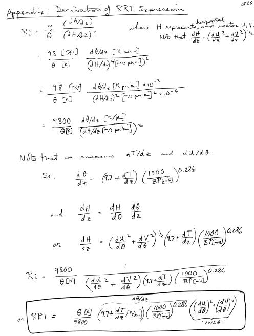
Note:  I've changed one number in this equation from it's original report value; I had used -10 [K/km] for adiabatic dT/dz, and in the present version I use -9.7 [K/km], which applies to an altitude of 10 km at a latitude of 30 degrees.

Explanatory note:  This work was funded by the Navy, supervised by Dr. Richard Siquig, on behalf of the High Altitude Long Endurance, HALE, aircraft that Boeing was building for possible reconnaisance use by the Navy.  This is a status report of my task to study the feasibility of using an MTP to guide the HALE away from CAT, so that the HALE platform could be stable for as much times as possible.  Shortly after submitting this report to the Navy the HALE project was cancelled.  I tried to interest NASA in continuing it, but NASA HQ had just undergone a transition of relying upon LaRC for guidance on what to fund.  By that time I had been "out of the loop" with NASA's aviation safety proram, and the new personnel at NASA HQ, and the people at LaRC, were unfamiliar with my previous NASA-funded CAT work.  Partly for this reason, I surmize, my CAT studies came to an end, and now languish with tantalizing leads left dangling!

One of my purposes in recording reports like this, which have never been published in the open literature, is to have them available for some future generation of investigators, and funders, who are genuinely interested in exploring a fuller understanding of the physics underlying the generation of CAT, and the aviation safety community who may be interested in solutions to the CAT safety problem.

Return to Main CAT Menu

This site opened:  Sep 19, 1999.  Last Update: Sep 19, 1999