The following is a description of an encounter with "moderate" CAT (Clear Air Turbulence) by NASA's ER-2 during its flight from Fairbanks, AK to Moffett Field, CA on 1991 October 14.  Values for Richardson Number, Ri, along the flight path are derived by combining MTP measured lapse rate with  the results of short timescale correlations of horizontal wind components with potential temperature.  The behavior of measured Ri support theories calling for Ri < 1/4 as a criterion for triggering CAT.  Both the Ri and lapse rate measurements are in accord with a simple model in which synoptic scale vertical compression produces a large region of high lapse rate (i.e., inversion layer) and low Ri, within which pockets of Ri < 1/4 eventually trigger CAT and destroy the inversion layer.  The measurements also support the prediction that each CAT patch, in addition to increasing the vertical separation of isentrope surfaces, converts air from Ri < 1/4 to air having Ri > 1.  These results are important in supporting claims that in the stratosphere observable properties of the air surrounding a patch of CAT can be used to predict the CAT encounter.

Introduction

This web page is intended for various investigators with an interest in the meteorology of CAT generation, and a selected few with an interest in CAT avoidance and prediction. If I later find the time to publish some of this data, it would be without the benefit of most of the figures, and the "asides" which serve to record my concerns and enthusiasms.

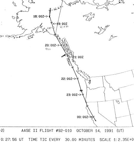
Ground Track

Figure 1 shows the flight track of the ER-2 during its 1991 October 14 flight from Fairbanks, AK to Moffett Field, CA. The region of interest for this report is southeastern Alaska, which is shown in the expanded map in Fig 2. The moderate CAT patch occurs  in  association  with  16,000-foot  Mt. Blackburn. Thus, the CAT is probably produced by mountain waves interacting with a pre-existing layer of high wind shear.

Figure 1.  Ground track of flight ER911014.  The CAT encounter occurred over southern Alaska.

Figure 2.  Close-up of ground track showing location of CAT encounter in relation to mountains.

Isentrope Altitude Cross-Section

Figure 3 is a curtain cross-section of isentrope surface pressure altitudes.  It was constructed from data taken by JPL's Microwave Temperature Profiler mounted in one of NASA's ER-2 aircraft, hereafter referred to as the MTP.  The "jumbled" region from 69 to 70 ks (kilo-seconds) is a mountain wave.  Figure 4 is a "zoomed" version of the mountain wave part of the previous isentrope altitude cross-section (IAC). The peak-to-peak vertical excursions of some isentrope surfaces is over 1000 meters. The isentrope pattern of vertical displacements exhibit horizontal wavelengths that range from 125 to 580 seconds, or 26 km to 120 km.

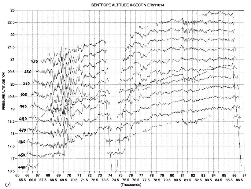
Figure 3.  Isentrope altitude cross-section, showing the large displacements early in the flight (at about 69 to 70 ks).

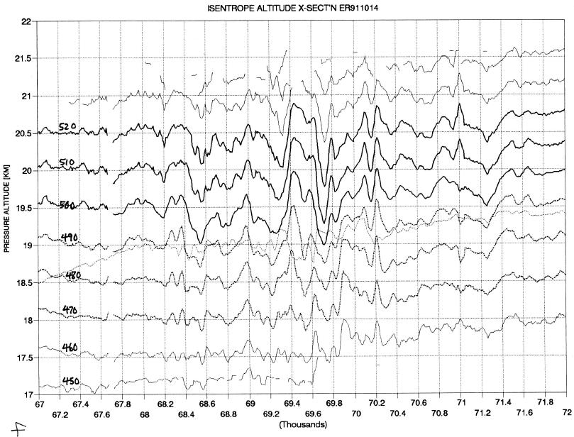
Figure 4.  Zoom of mountain wave region of previous figure.

Figure 5 zooms the previous IAC further, and shows the region of greatest isentrope altitude displacement. The flight path is shown by the thin "dotted" line. The vertical "hatching" on the flight path line shows where the MTP's vertical accelerometer exhibited large excursions in response to turbulence. The pilot, Jim Barrileaux, reported "moderate CAT about 200 miles east of Anchorage." He also reported encountering large temperature excursions, and he disabled the "auto-Mach hold" in order to fly the airplane manually.

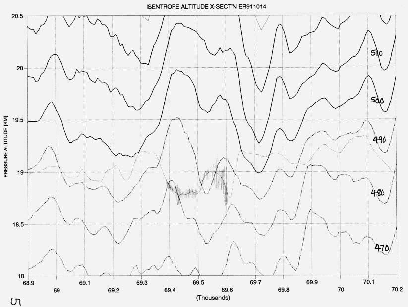
Figure 5.  An even closer zoom view of the previous figure, showing where turbulence was encountered (hashy structure along aircraft flight path).

Vertical Accelerometer Data

The upper panel in Figure 6 is a trace of the MTP's vertical accelerometer (a separate sensor from the aircraft instrumentation).  Readings are made at a rate of approximately 2.5 Hz. The accelerometer output is low-pass filtered at 20 Hz (half-response) before readings are made, so the readings are an under-sampled representation of the actual aircraft motion. The under-sampling is only a shortcoming when attempting to derive CAT intensity, as non-CAT flight does not contain significant vertical motions that require sampling at intervals less than 0.4 seconds.  An empirical correction for our under-sampling of the sensor has been established, so the data actually can be used to quantify CAT intensity.

Figure 6.  Vertical accelerometer (upper tace), lapse rate for a 500-meter thick layer centered on aircraft altitude (middle trace) and CAT intensity (lower trace).

The upper trace has two behaviors of note: KH waves, and CAT.  At 69.1 to 69.2 ks there are sinusoidal vertical motions with amplitude 0.25 g-units and a characteristic period of 19 seconds, or 4.0 km. I identify these to be Kelvin-Helmholtz waves, which are produced when vertical wind shear "overturning forces" approach the temperature field's "restoring forces."  KH waves grow in amplitude when the temperature field has insufficient vertical static stability to suppress vertical motions. Such waves usually occur in layers with high values of vertical wind shear and lapse rate.  A "rule of thumb" states that the horizontal wavelength of KH waves is approximately 7 times the layer's thickness. Accordingly, the 4.0 km wavelength "predicts" the presence of a 600 meter thick layer containing high wind shear and lapse rate. (More about this region later.)

The trace at the bottom, labelled "CAT INT," is the "5-second maximum of 1-second peak-to-peak of the accelerometer readings."  Since during CAT there is some "energy" at vertical motion frequencies higher than can be sampled by 2.5 Hz readings (but lower than about 15 Hz), the "CAT INT" lower trace will under-represent peak-to-peak excursions during periods of CAT.  I estimate that when CAT is present the CAT INT trace should be multiplied by 1.3. Thus, whereas the CAT INT trace reaches a maximum of 0.28 g-units (at 69.55 ks), a more frequent sampled version of our accelerometer output might have produced a CAT INT value of approximately 0.36 g-units.  This is generally considered to be within the range of "moderate" CAT.

Figure 7 shows a longer interval of accelerometer data.  Light CAT is generally considered to begin for peak-to-peak motions of about 0.10 g-units.  Allowing for the correction factor of 1.3, which should be applied to this data when CAT exists, we can place our threshold for light CAT at 0.07 gunits. Thus, there are light CAT encounters at 68.4 ks and 70.2 ks. The event at 69.92 ks appears to be an updraft, according to the upper trace, and should not be considered CAT. The slight feature at 69.1 ks can also be disregarded because it as an artifact of the CAT INT algorithm in the presence of large amplitude (non turbulent) waves.

Figure 7.  Same as previous figure except a larger span of time is shown.

Lapse Rate

The middle traces in Fig.'s 6 and 7 are MTP measured lapse rate, LR (defined here as the vertical gradient of temperature), for a layer 500 meters thick.  Referring to Fig. 7, the LR is generally isothermal (0 K/km), as is usually the case in the lower stratosphere. However, there is a 600 km region, from 68.4 to 71.4 ks, that includes high LR values.  It is quite rare to encounter LR as high as + 5 K/km at these altitudes, yet within this region such high values occur several times.

It is also unusual to encounter layers with LR as low as -5 K/km, yet such a region occurs at 69.4 to 69.6 ks, surrounded, ironically, by high LR air.  But the greater irony, and of course this is a meaningful clue to what is physically going on in this region, is that the very low LR air is located precisely with the moderate CAT patch.  This can be seen better in Fig. 6.  There is an almost perfect one-to-one correlation between CAT intensity and LR.  Note the abrupt ending of CAT at 69.6 ks, and the correlated abrupt LR transition from low LR to high values.  Note also the brief reduction of CAT intensity in the middle of the patch (at 69.5 ks) and the correlated brief rise in LR value.

Which is cause and which is effect?  CAT must cause the negative change in LR, as a complete mixing of air parcels in a region will necessarily produce adiabatic LR values (-10 K/km).  In going from +5 K/km to -7 K/km at the max-CAT time, the LR went approximately 80% of the way from its pre-CAT value (assumed, here, to be + 5 K/km) to the adiabatic value that a complete mixing would produce. Thus, the volume of air that was mature turbulence must have occupied at least 80% of the air volume sampled by the MTP instrument.  If the layer of CAT was limited to 600 meters thickness, and if this layer had a true LR of -10 K/km, then we can account for the measured LR by speculating that 20% of the MTP "antenna reception field" lay beyond the CAT layer. Given the geometry of this situation, this 20% value is possible.  I conclude that the low LR parts of maximum CAT intensity (at 69.44 and 69.55 to 69.6 ks) may have in fact produced an adiabatic LR.

Referring to Fig. 7, it is apparent that LR also goes negative at the times of the two light CAT encounters, at 68.4 and 70.2 ks. This light CAT produced LR values of -4 K/km versus the -6 or -7 K/km during moderate CAT.

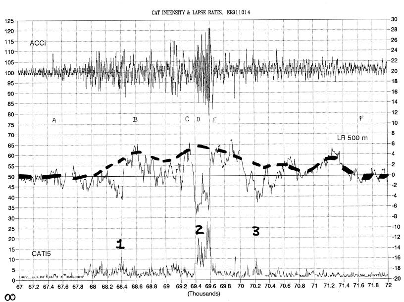
Figure 8.  Suggested pre-CAT lapse rate trace (middle) for encounters 1, 2 and 3.  Events "A" through "F" are identified here.

It will be instructive to imagine what the LR trace would have looked like before the CAT altered it.  Figure 8 is an attempt to do this.  In drawing the thick dashed line I was guided by the assumption that the greater the CAT the greater is the negative change in LR.  Thus, starting at 67.85, when "very light" CAT begins, the dashed line is slightly higher than the measured LR trace.  At the light CAT event "1" the LR dip is considered accounted for by continuing the dashed line upward.  Higher than measured values are sustained between "1" and "2" because very light CAT is present throughout this region.  The light CAT event "3" is allowed for in the same manner as for event "1."  What emerges is a large, synoptic scale region of elevated LR, extending from about 68.0 ks to 71.5 ks.  This region is 1.0 hour in extent, or 750 km.

These data further support my suggestion (Gary, 1991) that on a mesoscale LR is negatively correlated with CAT, whereas on a synoptic scale LR is positively correlated with CAT!

I would like to present a synoptic scale picture of what might be happening, for what it's worth (only qualfied meteorologists are allowed to snicker here).  I picture a synoptic scale air mass over-riding another, and the interface between them is slightly sloped.  The interface "layer" contains transitions in both wind vector and temperature.  The dynamics of the one air mass "sliding off" the other causes a thinning of the interface layer, analogous to losing "lubricant" between two solid objects with flat, sloped surfaces at their interface (it's obvious that I've never had a meteorology course).  The isentrope surfaces come together, as if under compression, and the isotach surfaces do the same.  The interface layer has more closely spaced isentropes, creating an inversion layer.  Synoptic scale processes continue to compress the interface region, bringing isentrope and isotach surfaces together.  I believe this is the scenario for the ER-2 flight under discussion, and by good luck the ER-2 was flying within the transition layer for 1 hour.  The existence of a mountain beneath the middle of this synoptic scale region of compression was another stroke of good luck, as it provided an additional distortion that brought isentrope and isotach surfaces together with the result that Richardson Number decreased an additional amount that was sufficient to trigger CAT.

Altitude Temperature Profiles

In Fig. 8 the symbols "A" through "F" indicate times for which "altitude temperature profiles" have been constructed.  The profiles are presented in Figures 9A through 9F.

Figure 9C and 9D.  Altitude temperature profiles, T(z), from the MTP instrument.  Each thin trace with small square symbols is an individual 14-second measurement, while the thick trace is an average of the group. Aircraft altitude is indicated by the "A/C" symbol.  The first profile group is "normal" or "undisturbed."  The second group exhibits a dramatically rapid vertical compression, creating an inversion layer due to adiabatic heating.

Figure 9A is "normal" in the sense that no inversion layer temperature structure is present. The lapse rate is indeed isothermal at flight level (18.75 km), which is consistent with the LR trace in Fig. 8. Figure 9B shows the presence of a strong and shallow inversion layer at flight level, FL. Note that the inversion layer is about 500 meters thick, and that compression is a likely origin due to the fact that the two profiles are identical below FL but warmer than in Fig. 9A above FL. The maximum temperature difference is 3 K (at 19.5 km), implying a vertical descent (compression) of 300 meters.

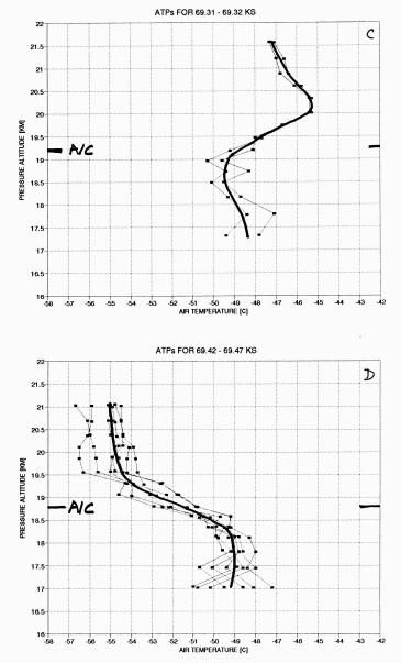
Figure 9C and 9D.  This pair of T(z) groups are from "just before" to "within" a CAT patch.  Notice how the mixing of air by CAT motions has converted an inversion layer into an almost adiabatic layer.

Figure 9C is immediately before the moderate CAT event, and this profile shows the maximum amount of "warming."  The air at 20 km is 5.7 K warmer than the air at the same altitude in Fig. 9A. This could be interpreted as a 570 meter descent if it can be assumed that the air at location "C" originally had the same temperature profile as in "A." Note that the inversion layer is 1000 meters thick at "C."

Figure 9D is for a time only 2 minutes after the profile in the previous panel.  At 20 km the air is 9.5 K cooler at "D" than at "C"!  The air below FL is unchanged.  If it is assumed, for the moment, that mountain waves were not moving air up and down in a non-mixing, reversible process, then by overlaying panels 9C and 9D, and drawing adiabat lines between the two profiles, it is possible to account for the colder temperatures at 20 km by hypothesizing that the redistribution of air produced by turbulence caused air that originally was at 19.4 km to end up at 20 km.  Continuing with this assumption that mountain waves are not present, the turbulence redistribution would have to extend from 18.5 km to higher than 22 km.  This strikes me as a tremendously thick layer for CAT, and shows that it is necessary to allow for the mountain wave motion before calculating altitude redistribution statistics.

Figure 9E and 9F.  Another illustration of the temperature field immediately outside a CAT patch (upper) and a distant location apparently not undergoing vertical compression by synoptic scale forces.

Figure 9E is for a time immediately after the abrupt cessation of CAT.  An inversion layer is present which is somewhat similar to the pre-CAT inversion layer in Fig. 9C.  Inversion layer thickness is about 1000 meters, but the altitude of the layer is about 800 meters lower at "E" compared to "C."  The aircraft went from flying near inversion layer base, at "C," to flying near inversion layer top, 6 minutes later at "E."  These comparisons support the notion that the interface (compression) region is sloped.  Figure 9F is for "normal" air, and shows that beyond the 600 km "compressed" region, from 68.4 to 71.4 ks, inversion layer structures are not present.

Tentative Richardson Number Derivation

Appendix A contains a complete description of the procedure I have used to estimate Reciprocal Richardson Number, RRi.  The procedure is tentative because it rests on the validity of one key assumption which may not be meteorologically sound.  Part of this exercise is to evaluate the soundness of this assumption by comparing the behavior of "measured" RRi with behaviors that meteorology theory predicts. Thus, if RRi varies in the expected way before, during, and after a CAT event, then this might constitute evidence that RRi had indeed been correctly derived, and that the questionable assumption was justified.  In the process of all this hypothetical RRi comparison, it may actually be possible to gain insight into CAT generation.

In any case, it should be possible to evaluate the merits of developing empirically useful techniques for predicting CAT encounters using whatever it is that "measured flight path RRi" is a measure of.  If "measured flight path RRi" is actually a measure of something else (related to actual RRi), then it may still be a valuable parameter, as it might have predictive capability.

The appendix can be skipped by most readers; it merely describes a way of correlating the U and V components of horizontal wind  with  potential  temperature, theta.   The correlations are performed for data chunks with lengths that are typically 30 seconds. Variations of theta occur due to a combination of aircraft altitude fluctuations (of order 8 meters, RMS, during 30-second intervals) and flight through a wrinkled pattern  of  isentrope  surfaces (producing  theta fluctuations of order 15 meters, RMS, during 30-second intervals).  Each data chunk produces empirically determined parameters which I will call dU/dtheta and dV/dtheta.  These are multiplied by dtheta/dz, which the MTP instrument measures, yielding estimates of dU/dz and dV/dz.  The orthogonal sum of these two gradients is an estimate of "vertical wind shear," VWS.  Knowing VWS and dtheta/dz (closely related to lapse rate), it is possible to calculate Richardson Number, or its reciprocal RRi.   If you're satisfied with this explanation for measuring RRi, then you may skip the appendix.  Still, keep in mind that although the RRi plots that follow are tentatively identified with actual RRi, they really bear an unknown relation to RRi because of the one questionable assumption, described in the appendix.

Richardson Number Behavior

Since the Reciprocal of Richardson Number, RRi, is never used in the literature, I will first review the relationship of Ri to CAT generation so that the reader who is familiar with Ri can compare our respective understandings of Ri's relation to CAT.

Most of the atmosphere consists of Ri >> 1, such as 5 or 10.  According to meteorological models for the growth and breakdown of Kelvin-Helmholtz waves, Ri < 0.25 is a necessary (though not sufficient) condition for the breakdown of the KH waves (and a subsequent generation of CAT).  CAT, once initiated, grows throughout the altitude region where Ri < 1, and the resultant mixing causes this region to take on values of Ri > 1.

Stating this in terms of RRi, as preparation for the figures that follow, the typical atmosphere has RRi << 1, such as 0.1 or 0.2.  When RRi > 4 it is possible for KH waves to undergo breakdown, and generate CAT.  The CAT will grow throughout the altitude region where RRi > 1.  CAT, once started (where RRi > 4), will thus convert the entire layer of air that has RRi > 1 to air with RRi < 1.

As additional preparation for the figures that follow, consider the case of one synoptic scale air mass, such as 600 km wide, over-riding another air mass.  Assume that the shallow interface between them contains a greater amount of wind shear than exists within either air mass.  There often is a slight temperature inversion at the interface between the air masses.

If, for any reason, the interface region becomes shallower, the isentrope surfaces will come together and the interface LR will increase.  This could cause the interface region to become an inversion layer (if it is not already one). The isotach surfaces (surfaces of constant horizontal wind speed) may also come together in the same way.  If this happens, then the vertical gradients of potential temperature and horizontal wind will increase in the same proportion.  Since RRi is proportional to the square of the wind gradient, but only the first power of the potential temperature gradient, RRi will change, becoming larger.  If it increases to 4, the scenario for CAT generation may commence.  Inversion layers are thus favored sites for generating CAT.

Is there evidence in this flight segment's RRi data that these things were occurring?

Yes!  Figure 10 is a plot of RRi, showing a 30-second weighted average trace, which I shall refer to as RRi30.  A Gaussian-weighted (FWHM = 105 second) average trace will be referred to as RR130/105.  Approximately 5 minutes before the moderate CAT encounter the RRi30/105 trace rises to about 3.  During CAT, RRi30/105 decreases to about 1.  After the CAT, RRi30/105 rises again to about 2.5.  Recall that since the layer undergoing compression is shallower than the altitude region sampled by the MTP measurements, we should
expect to see slightly smaller values for RRi than actually are occurring within the layer.  Thus, where RRi appears to be 3 it could actually be 4 within the layer.

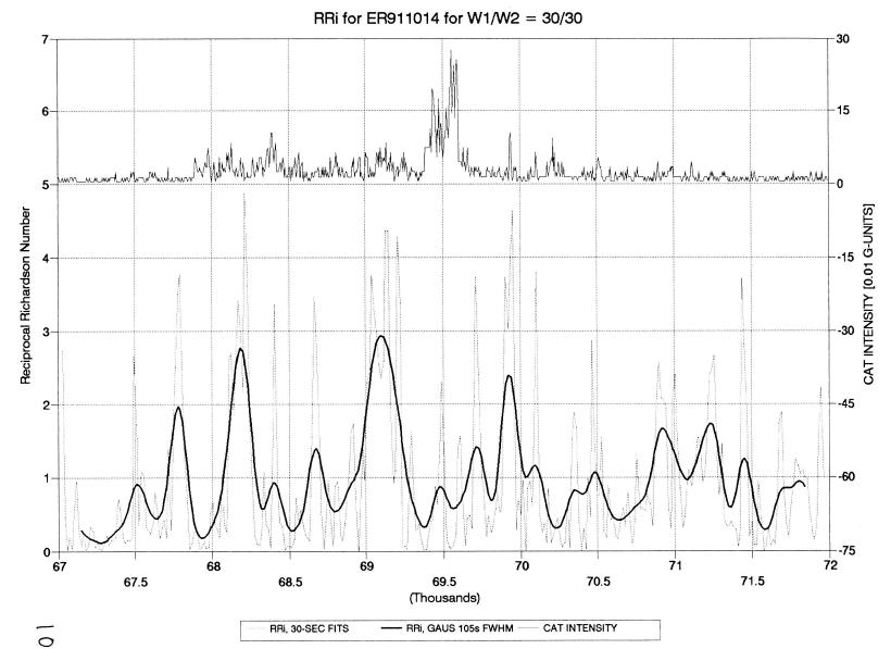
Figure 10.

What about the two light CAT encounters?  The first light CAT encounter, at 68.3 ks, is preceded by RRi30/105 rising to almost 3.  During the CAT RR130/105 falls to about 1.  The rise of RRi afterwards is not present. The second light CAT encounter, at 70.2 ks, occurs when RRi is below 1.  It is preceded by the high RRi that follows the moderate CAT event, so it is not possible to state that it is preceded by high RRi.  It is not followed by high RRi, however, according to the RRi30/105 trace.

It is noteworthy that the RRi30 trace approaches 4 several times, but never exceeds the value 4 by very much (usually 4.5, once 4.9).  These behaviors are consistent with Ri theory, since RRi must exceed 4 within the CAT-generating layer for an unspecified time required for amplitude growth to reach a state of instability.  Again, the values of RRi plotted here should be thought of as under-estimates due to the shallowness of the layer being measured in relation to the long weighting function of the MTP measurements.

The interval 69.0 to 69.2 ks is noteworthy in appearing to have a robustly high value for RRi.  All but one of the 12 values of RRi30 within this interval are greater than 2.  Referring to Fig. 6, this is the time when high amplitude KR waves are present.  According to the values of RRi30 during the waves, breakdown might have been immanent for them.  If the waves underwent compression, producing high lapse rates (note that LR is isothermal, here), RRi would probably increase, thus enhancing the prospects for CAT.  Farther along the flight path this increased "compression" may have occurred, as shown by the high LR, and within the moderate CAT segment RRi must have originally been high enough, and lasting long enough, to have triggered KR wave breakdown and CAT.

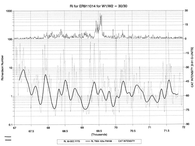
Figure 11.  Same as prevous fiure, except that Ri is plotted (on a log-scale) instead of RRi.

Figure 11 is the same data plotted as Ri instead of RRi.  Occasional very high values of Ri are easy to produce in the presence of measurement noise when the true value of Ri is high, since VWS = 0 produces Ri = infinity.  It is for this reason that I prefer RRi.  Note that the averaging is still of RRi30, not Ri30.  Presumably, the high Ri values (5 or 10) at the beginning of the plot are typical of the undisturbed atmosphere.

Control Data Analsys

To test the assumption that "undisturbed" air exhibits less dramatic LR variations than appear in Fig.'s 6 - 8, and lower RRi traces than appear in Fig. 10, the same analysis that has just been described was performed on a "control" flight segment, the last 3000 seconds of this same flight.

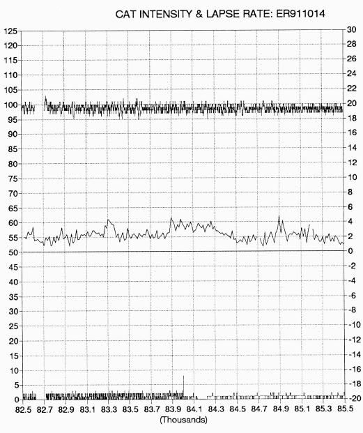
Figure 12.  Same analysis performed on "control" data, showing that the accelerometer record (top), lapse rate (middle) and CAT intensity (bottom) are "uneventful."

Figure 12 is the control data counterpart of Fig. 7, and has identical horizontal and vertical scales. It shows accelerometer, CAT intensity, and LR data for the interval 82.5 to 85.5 ks. This control data shows that there are no KR wave structures, no CAT encounters, and no LR variations.

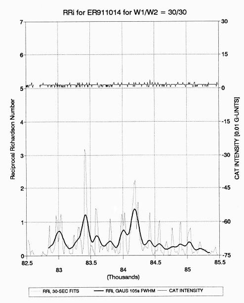
Figure 13.  RRi analysis for the control data.

Figure 13 is the control data counterpart to Fig. 10, and has identical horizontal and vertical scales. It shows RRi30 and RRi30/105 for the 82.5 to 85.5 ks interval. This control data shows that there are no RRi30 events > 4, and no RRi30/105 events > 2 (the threshold used in an example algorithm, below, for predicting moderate CAT encounters). The average RRi is 0.3 (i.e., the average Ri is 3).

The control data provide reassurance that the LR and RRi features noted for the data interval that includes a moderate CAT encounter are not found during smooth flight segments.  I can assure the reader that abrupt changes of LR, such as from + 4 to -5 [K/km], are extremely rare.  As time permits, more control data will be analyzed to strengthen the claim that "measured flight path RRi" is almost always < 2, and typically << 1, during periods without CAT.

CAT Warning Algorithm

The data  presented  here  suggests  that  a combination of RRi and LR appear to be essential inputs to any algorithm that endeavors to predict CAT encounters.  Nevertheless, it will be instructive to first consider algorithms based on just one observable at a time.

If only LR were available, and if it could be measured well ahead of the aircraft, there might be merit in an algorithm that alerts when LR goes abruptly from high to low.  Such an algorithm would have predicted the moderate encounter going in both directions.  Presumably, only CAT can "wipe out" an inversion layer abruptly.  Inspection of Fig. 6 shows that LR began to fall significantly before CAT increased to significant levels during ingress, whereas during egress from CAT, LR increases at exactly the same time as CAT intensity subsides (according to this plot, with 9-second  LR resolution).  An MTP with a much lower frequency channel might be employed to measure lapse rate at a farther distance from the aircraft.

(Many years ago, while flying the MTP/C141 instrument, I noted a phenomenon which I referred to as "tropopause washout."  CAT was associated with tropopauses that abruptly lost their sharp temperature field structure, such as going from a tropopause with a marked coldest temperature altitude to one that I referred to as a "soft tropopause."  This phenomenon, if verified by more data, would surely be analogous to the "inversion layer washout" noted here.)

Using RRi by itself would produce alarms for light and moderate CAT indiscriminately, according to my reading of Fig. 10.  For example, if a RRi30/105 threshold of 2 were used for predicting CAT, there would be 3 warnings for this data.  Two would have been for light CAT, and only one would have been followed by moderate CAT.  At least CAT of some intensity would have followed each warning.  For this assessment to be meaningful it will be important to analyze more than the 48-minute "control data"  of smooth flight conditions to be sure that smooth air does not produce false alarms using CAT warning algorithms of this report.

Combining RRi and LR may afford improved CAT warnings.  For example, consider the following algorithm:

With this algorithm there would have been one moderate CAT prediction, and it would have been accurate.  Note that a "however" qualifier will be necessary for any good warning algorithm, since it is a desirable feature that every CAT patch should look the same flying out of it as flying into it.  Thus, this warning algorithm would have been just as successful "flying backwards" through this data as "flying forward" through it.

I would like to suggest that the apparent agreement of the RRi data with basic KH wave growth and breakdown theory argues that the "flight path RRi algorithm" is producing a product that is at least closely related to RRi, if in fact it is not a valid measure of RRi.

As I argued in another report (Gary, 1991), any serious effort to derive warning algorithms should rely upon multiple regression analyses of many observables and quasi-observed parameters (such as RRi).  In this way, explicit use can be made of all easily measured atmospheric properties, in accordance with empirical correlations.  The role of meteorological insight is then one of designing the architecture of the warning algorithm and creating quasi-observables  (out of directly measured observables) that "should" have warning potential.

Summary

Lapse rate was found to exhibit a striking correlation with turbulence intensity during an encounter with moderate CAT.  During CAT, lapse rate abruptly approached adiabatic, implying that either 1) the CAT led to >80% vertical mixing of air within the layer that generated the CAT, or 2) the completely mixed CAT layer "filled" >80% of the MTP weighting function for viewing angles used to derive lapse rate.  Two light CAT encounters were also associated with drops in lapse rate.  All CAT encounters are within a synoptic-sized (750 km long) region of enhanced LR which appears to have been caused by a downward motion of the overlying air mass which in turn led to adiabatic heating sufficient to produce the observed inversion layer at the air mass interface.

A method for attempting to infer Reciprocal Richardson Number, RRi, along the flight path has been demonstrated.  This "measured flight path RRi" approaches 4 on several occasions, and is persistently close to 4 prior to a moderate CAT encounter.  The fact that the behavior of "measured" RRi during a CAT encounter agrees with predictions from a simple model suggests that something closely related to RRi, is, in fact, being measured by the "flight path RRi algorithm."

The present analysis of a moderate CAT encounter supports my position, stated in previous reports (such as in Gary, 1991), that CAT patches are surrounded by a "doughnut" shaped region which contains information which, if properly interpreted, reveals the existence of the turbulence within.  The task at hand is to figure out how to fully interpret what the doughnut is trying to tell us.

Acknowldgements

The "measured flight path RRi" analysis could not have been performed without the horizontal wind measurements of the Meteorology Measurement System, MMS, aboard the ER-2.  I thank K. Roland Chan, the MMS Principal Investigator, and his colleagues, for making this data available.

References

Gary, B. L. (1991), "Clear Air Turbulence Avoidance System for the HALE Aircraft," Naval Oceanographic and Atmospheric Research Laboratory, Technical Note 194, November 1991.

Richardson Number can be approximately thought of as the ratio of temperature field stabilizing "forces" to wind shear driven overturning forces.  I prefer use of Reciprocal Richardson Number, RRi, as there are better properties when averaging noisy estimates of RRi than noisy estimates of Ri. RRi is:

    RRi = (theta/g)*(dz/dtheta)*VWS²

where theta is potential temperature [K], g is the earth surface gravity constant, 9.80 [m/s²], z is geometric altitude [m], and VWS² is the square of vertical wind shear [s^-2] For completeness,

    theta  = T [K] * (1000/BP[mb])^0.286

where T [K] is air temperature, and BP [mb] is barometric pressure at flight altitude.  Also,

    dtheta/dz = (dT[dz + 10)*(1000/BP)^0.286

Whereas dtheta/dz = geometric lapse rate, the MTP instrument measures pressure altitude lapse rate, LR, which is the vertical gradient of air temperature with respect to pressure altitude, Zp.  One lapse rate can be converted to the other by noting that

    dZp/dz = (Tstd [K] / T [K]),

where Tstd [K] is the U. S. Standard Atmosphere temperature for the pressure altitude of the aircraft.

Thus,

    LR = dT/dZp,

    dT/dz = LR * (Tstd [K]/ T [K]}.

VWS is the magnitude of the vector difference of winds at two closely-spaced altitudes.  Thus,

    VWS² = (dU/dz)² + (dV/dz)²

where U and V are the eastward and northward components of horizontal wind, which are measured by the Meteorology Measurement System, MMS (in this study).  It is not possible to directly measure the vertical gradients of U or V.  However, due to slight vertical motions of the aircraft, and ever-present slight vertical displacements of small air parcels (of size 1 to 5 km), it is possible to directly measure something tantalizingly close to the vertical gradients:

    dU/dtheta and dV/dtheta.

If we had a true measure of the gradients of U and V with respect to theta then we could convert them to gradients with respect to z by the following multiplication:

    dU/dz = (dU/dtheta) * (dtheta/dz),
    dV/dz = (dV/dtheta) * (dtheta/dz),

where dtheta/dz is derived above.  Thus, provided it is possible to somehow obtain a measure of dU/dtheta and dV/dtheta, all parameters needed to calculate RRi would be available.

Bringing together the above derivations, we can write an equation for RRi:

    RRi = (theta/g) * (10 + LR*Tstd/T) * (1000/BP)^0.286 * {(dU/dtheta)² + (dV/dtheta)²}

where LR is measured by the MTP instrument once every 9 seconds and U, V and theta are measured by the MMS instrument every second.  The crucial question for this process rests on the weakest link in the entire chain of reasoning, namely:

Is it possible to obtain a reliable measure of dU/dtheta and dV/dtheta by correlating U and V with theta?

The meteorologists I have queried are unanimous in feeling uncomfortable with the assumption that an in situ correlation of U and V with theta, over any timescale, is the same as dU/dtheta  and dV/dtheta.  The two would be equal if air parcels did not move vertically, and only the aircraft moved up and down; in effect, sampling a horizontally stratified temperature and velocity field.  Approximately 1/3 of the flight path's sampling of air is of this type.  The aircraft's pressure altitude typically exhibits fluctuations of order 8 meters, RMS (30 meters, peak-to-peak) during 30 second intervals. However, a greater amount of theta fluctuations occur due to the wrinkled structure of isentropes.  For 30-second intervals, a level-flying ER-2 aircraft will experience theta fluctuations due to isentrope wrinkling having RMS values of about 15 meters (60 meters, peak-to-peak). These values are for non-CAT air. During flight in mountain wave air these values can approximatley triple.  As a rule, the isentrope altitude fluctuations are twice the ER-2 altitude excursions.  As air parcels move up and down 10 or 15 meters from their mean altitude, do they retain their mean horizontal wind vector?  If they do, then it would be possible to adopt the assumption that there is an equality of 30-second correlations of U and V with theta and the mean field's dU/dtheta and dV/dtheta at one ground track location, and then proceed to calculate RRi according to the procedure outlined above.

I am unable to evaluate the merits of making the crucial assumption that the correlations of U and V with theta are approximately equal to dU/dtheta and dV/dtheta, so I have taken the following position.  I will tentatively assume that they are equal, and use RRi derived under this assumption to see if it is consistent with predicted behaviors for the RRi of theoretical meteorologists.  If the questionable assumption is OK, then my "measured' RRi should bear specific relationships to CAT encounters.  Namely, CAT should be preceded, and followed, by RRi ~ 4, active CAT patches should have RRi < 1, and regions with no CAT nearby should have RRi << 1 (such as 0.2).

The details of how I have chosen to correlate U and V with theta are worth describing.  It is necessary to minimize the influence of horizontal gradients of U and V when calculating the correlation of U and V with theta.  The process begins with a 1-second resolution time series of U, V, and theta.  A "chunk" of data, such as 30 seconds long (W1 = 30 seconds), is chosen for a least squares analysis.  A simultaneous LS solution is performed for U with time and theta, and the same for V with time and theta.  This can be done for the next 30-second chunk of data, etc, until the end of the entire data set.

The set of correlations corresponding to dU/dtheta and dV/dtheta could then be adopted for use in the algorithm for RRi given above.  However, a better result is obtained if the entire process is repeated for offsets of I second, 2 seconds, etc, to 29 seconds (if 30-second chunks were used).  If the results are arranged by starting chunk time, then some form of averaging can be performed to produce a manageably small set of theta-gradient results.

An averaging procedure has been developed that performs a weighted average of the sequence of 1-second offset LS solutions for dU/dtheta and dV/dtheta.  The averaging interval is W2 seconds, and weighted averages are calculated every 0.5 * W2 seconds (some structure in weighted average result would be lost if intervals longer than 0.5 * W2 are used).  W2 values in the range 20 to 60 seconds have been evaluated for several WI choices.

To obtain one weighted average, each of the W2 1-second LS results for dU/dtheta and dV/dtheta is assigned a weight according to the following equation:

    Weight = 1/{(1+(HG/4)² + (RMSf/25)²}

where HG is the horizontal gradient, either dU/dt or dV/dt [m/s], and RMSf is the final RMS [m/s] off the 2-dimensional LS fit.

By using a weight of this form the weighted average gradient of U or V with theta will be influenced more by data chunks in which:  1) theta changes could be represented well by the linear fits, and 2) horizontal gradients were small.  (The constants 4 and 25 were chosen through a process of combining judicious estimations with trial and error runs, using a 3.6-hour segment of the ER-2 flight of 1998 December 29, described in Gary, 1991.)

It makes sense to choose W2 about equal to W1.  For these cases, every second weighted average U and V gradient with theta is "independent" of all others.  Most of my analyses have adhered to this practice.

The above amount of averaging  provides independent estimates of RRi every W1 seconds.  Values for W1 between 20 and 60  seconds have been evaluated.  In plotting VWS values versus W1, there is a broad maximum at W1 = 30 seconds (a broad maximum was also present for Wl ~ 30 seconds  for  the 1998 December 29 data).  Presumably, this interval affords the best trade-off of wanting large theta ranges (for producing strong LS solutions of the dependence of U and V on theta) and wanting short horizontal distances (for minimizing the contaminating effect of horizontal gradients).

The sequence of RRi values, with (typically) 15-second spacing, are shown in all presentations of this report.  However, these RRi data show large variations.  Although the variations may be real, they do not lend themselves to visualizing trends.  Thus, another level of averaging has been imposed.  Triangular-weight-averaging has been employed in a spreadsheet analysis format.  When a second column of triangular-weight-averaging is applied to the first, a close approximation to Gaussian weighting of the original data column is achieved (whose full-width/half-maximum, or FWHM, is 1.4 times the FWHM of the first triangular weighting column).  When W1 = W2 = 30 seconds, a Gaussian weighting with FWHM = 100 seconds produces a "pleasing" result.
~~~~~~~~~~~~~~~~~~~~~~~~~~~~~~~~~~~~~~~~~~~~~~~~~~~~~~~~~~~~~~~~~~~~

Link Back to CAT Overview web page.
____________________________________________________________________

This site opened:  1999 August 22.  Last Update: 1999 August 25