RA/DE = 21:13:46.04 +26:21:28.4 (measured on 20110829 by Gary)
V ~ 14.7, B-V = +0.24, CMC14 r' = 14.72, J = 14.230 (36), K = 14.095 (57)
Period Coverage
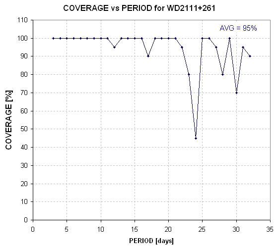
Figure 1. Coverage versus period.
Thoughts on Where Things Stand for This Target
We should keep in mind that for this WD there are no cases of LC overlap. Therefore, any speculation based on the presence of quasi-sinusoidal variations, found in several of the uncorroborated LCs, will be resting on a belief that LC variations don't require corroboration to be believed. This belief can be based on the presence of similar variations (amplitude, period and phase) for all LCs with sufficient precision to show the hypothesized variation. Any variation that is not present in this manner, such as non-periodic variations (different amplitudes, or different periods, or no consistency with a fixed phase) will require overlapping LCs exhibiting the same structure before they can be considered real. The highest priority goal for this target is to provide overlapping LCs with good precision.
The following two plots were constructed when I was optimistic that WD2111+261 was variable. They assume a constant period and amplitude. Most observations reported so far have been made using either a clear filter or a "clear with blue-bocking" (Cbb) filter, I assumed that all LCs could be combined using a phase-folding analysis. However, all Harvard-Clay observations are mae with an R-band filter, and this might account for their higer than others amplitudes.
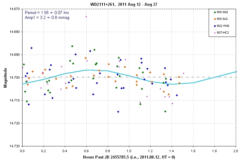
Figure 2. Phase-folded LC for the best fitting sinusoid (amp = 3.2 ± 0.8 mmag, P = 1.55 ± 0.07 hr). N = 103. Based on data up to 20110827.
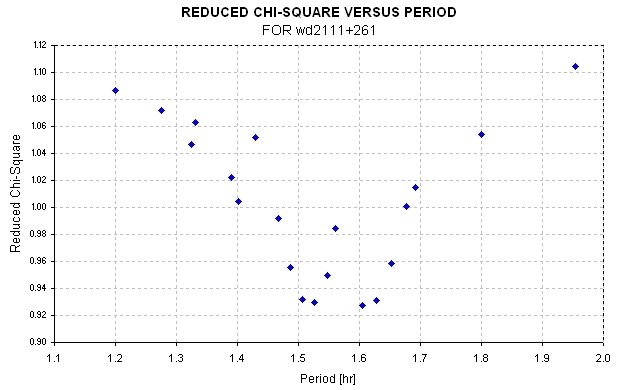
Figure 3. Reduced chi-square versus period (for each period all other parameters are optimized). N = 103, so chi-square increases by 1.0 when reduced chi-square increases by ~ 0.01. Based on data up to 20110827.
It is my impression that the "sinusoidal" variation (if it exists) is really just "quasi-sinusoidal" since the period doesn't appear to be constant. But if the variations are sinusoidal, and the period is constant, then the above phase-folded analysis is the best "solution" (assuming the minimum chi-square solution that I found is a "global" solution).
One further thought (that may be discomfitting): There appears to be a relationship between the fitted sinusoidal amplitude and light curve noisiness, as illustrated by the following plot.
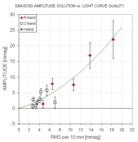
Figure 4. Fitted sinusoid amplitude versus noisiness of light curve, symbol-coded by filter band.
The correlation of amplitude with noisiness is obvious, but what about amplitude versus filter band. One of the lowest noise LCs was made with a R-band filter, and the longest wavelength (I-band) exhibited an amplitude that is less than three R-band LCs. Therefore, the inital impression that only the R-band LCs had large amplitude variations is no longer true for this object.
If there's something about the processes of observing, image analysis and photometry that produces spurious quasi-sinusoidal variations (timescales of hours) at the same time that it produces noisy LCs (timescales of minutes), then this finding should exist for other target stars. Is there evidence for that?
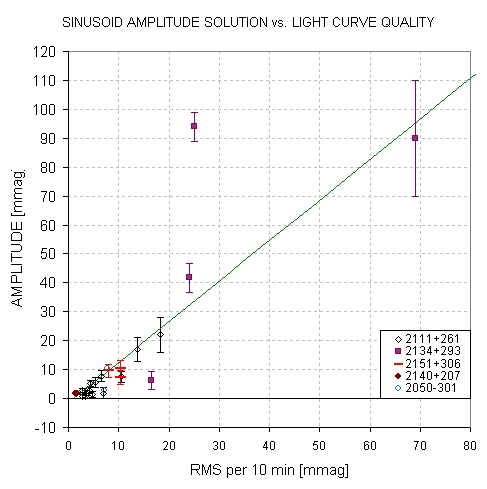
Figure 5. Fitted sinusoid amplitude versus noisiness of light curve for all PAWM targets for which sinusoidal fits were made (as of 2011.08.30), first notd by Howard Relles and subsequently added to by B. Gary.
The answer is "yes" - at least 23 of the 24 cases can be fitted by the equation:
Spurious Sinusoidal Amplitude = 1.4 × (RMS10 - 1 mmag)
where RMS10 is the RMS precision for 10-minute intervals, based on a neighbor differences analysis. If this relationship is used to reject LCs as having a real quasi-sinusoidal variation, then only one case should be considered a candidate for exhiting a real variation (Srdoc's 2011.08.17 observation of WD2134+293).
There's one final speculation that, for completeness, should be considered. Whenever an inexperienced observer observes a target star the star increases its real variation amplitude. This cannot be true because on several occasions observers with differing experience (as measured by RMS10), while observing at about the same time, produce LCs that exhibit greatly differing amplitudes.
I am currently preparing a description of the problem of spurious sinusoid amplitudes versus LC noisiness, that includes a theoretical confirmation (prepared by Prof. Eric Agol) of the empirical relationship from PAWM LCs: http://brucegary.net/WDE/WDcatchall.html#Spurious_Sinusoidal_Amplitude_Problem
Given the above relationship between fitted sinusoid amplitude and light curve noisiness there is a suggestion that perfect data, with no noise, would show a zero amplitude variation. This would imply that all other variations on this web page are not real. Perhaps the real message of the above plots is that it is prudent to adopt the default position that non-overlapping light curves should be used with extreme caution to infer the presence of real sinusoidal variations, and only overlapping LCs showing the same structure are acceptable evidence for variability. This is why I've been trying to coordinate European and USA observers to coordinate their observations of this target until we know how much to believe the uncorroborated LCs that show variability.
Listing of Observations
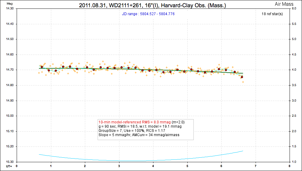
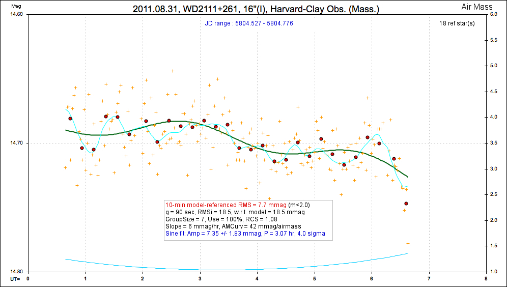
20110831 6.0 hrs 5804.527 - 5804.776 I Harvard-Clay Smooth, RMS10 = 7.7 mmag, sine: 7.4 ± 1.8 mmag, P = 3.1 hr, 4.0 sigma
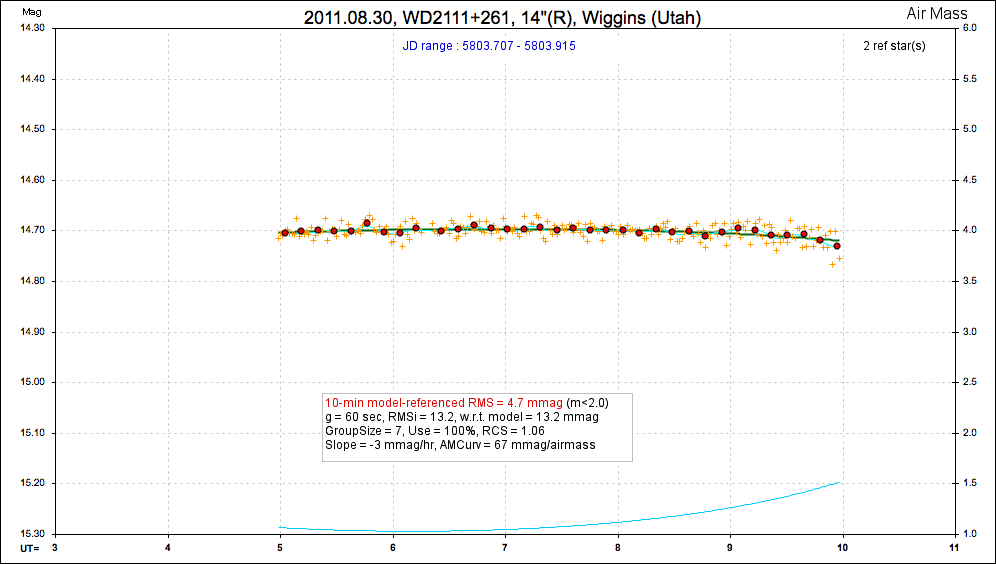
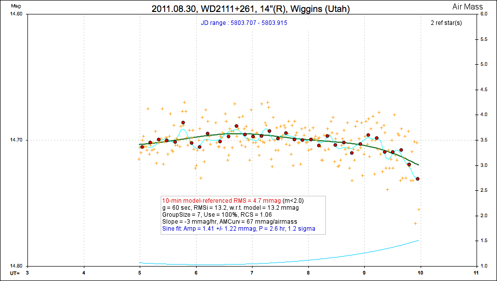
20110830 5.0 hrs 5803.707 - 5803.915 R Wiggins Smooth, RMS10 = 4.7 mmag, sine: 1.4 ± 1.2 mmag, P = 2.6 hr, 1.2-sigma
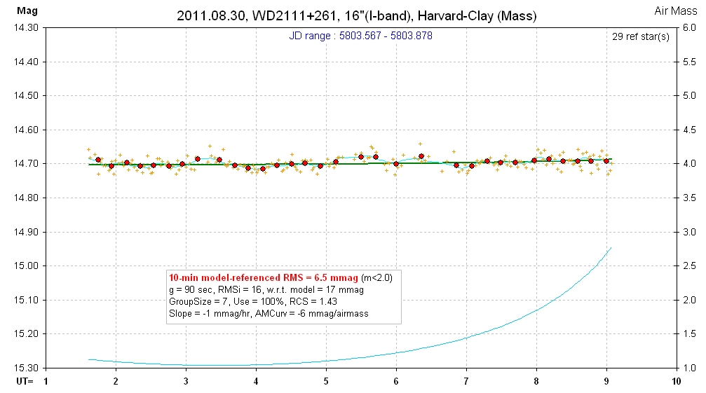
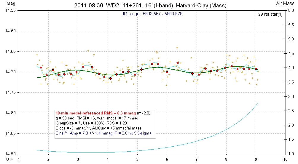
20110830 7.5 hrs 5803.567 - 58.3.878 I Harvard-Clay Smooth, RMS10 = 6.5 mmag, sine: 7.8 ± 1.4 mmag, P = 2.8 hr, 5.5-sigma
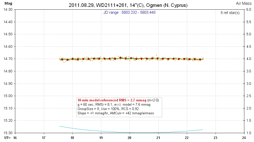
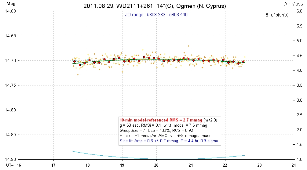
20110829 5.0 hrs 5803.232 - 5803.440 C Ogmen Smooth, RMS10 = 2.7 mmag, sine: 0.6 ± 0.7 mmag, P = 4.4 hr, 0.9-sigma
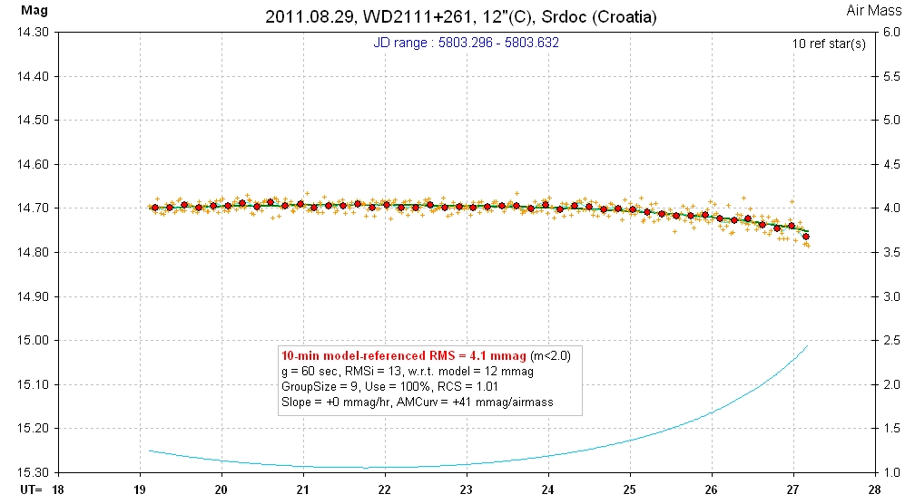
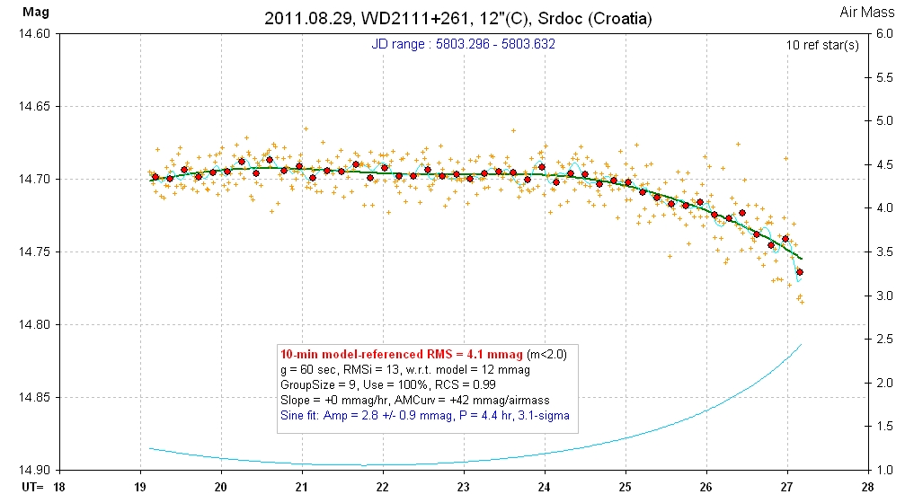
20110829 8.0 hrs 5803.293 - 5803.632 C Srdoc Smooth, RMS10 = 4.1 mmag, sine: 2.8 ± 0.9 mmag, P = 4.4 hr, 3.1-sigma
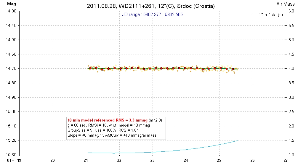
20110828 4.5 hrs 5802.377 - 5802.565 C Srdoc Smooth, RMS10 = 3.3 mmag, sine: 0.8 ± 0.9 mmag, P = 2.3 hr, 0.8-sigma
20110829 7.0 hrs 5802.588 - 5802.873 C Vander Haagen Smooth, RMS10 = 7.0 mmag, sine: 1.9 ± 1.8 mmag, P = 2.7 hr, 1.8-sigma
20110829 9.4 hrs 5802.612 - 5803.005 Cbb Gary Smooth, RMS10 = 2.9 mmag, sine: 2.8 ± 0.6 mmag, P = 2.9 hr, 5.1-sigma
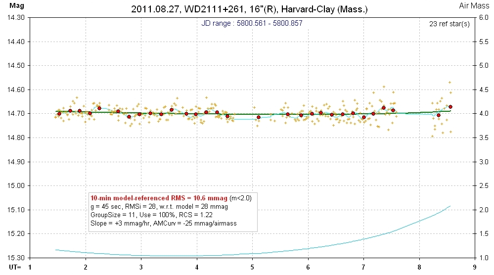
20110827 7.0 hrs 5800.561 - 5800.857 R Harvard-Clay Smooth, RMS10 = 10.6 mmag, sine: 7.5 ± 1.9 mmag, P = 1.8 hr, 3.9-sigma
20110822 7.2 hrs 5795.566 - 5795.868 C Vander Haagen Smooth, RMS10 = 4.3 mmag, sine: 5.3 ± 1.1 mmag, P = 2.4 hr, 4.8-sigma
20110817 7.1 hrs 5791.375 - 5791.669 C Gregorio Smooth, RMS10 = 3.6 mmag, sine: 1.9 ± 0.8 mmag, P = 1.6 hr, 2.3-sigma
20110813 4.0 hrs 5786.585 - 5786.753 R Harvard-Clay Smooth, RMS10 = 13.8 mmag, sine: 16.9 ± 4.1 mmag, P = 2.0 hr, 4.1-sigma
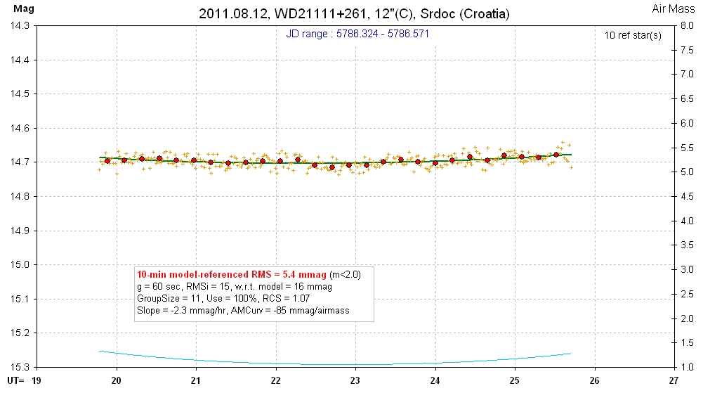
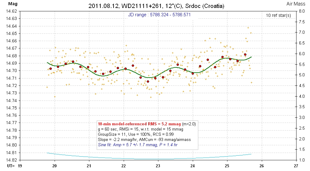
20110812 5.9 hrs 5786.324 - 5786.571 C Srdoc Smooth, RMS10 = 5.4 mmag, sine: 5.7 ± 1.7 mmag, P = 1.4 hr, 3.4-sigma
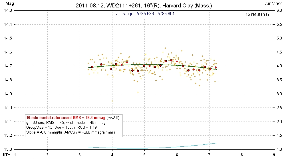
20110812 4.0 hrs 5785.636 - 5785.801 R Harvard-Clay Smooth, RMS10 = 18.3 mmag, sine: 22 ± 6 mmag, P = 1.7 hr, 3.6-sigma
Light Curves
For all of the following light curves I'll present at least two plots; one with a 1.0 mag range and another with an expanded mag scale for showing a sinusoid fit. The fit is obtained by manually setting the amplitude, period and phase for approximate agreement with data, then allowing a chi-square minimization to proceed (Excel "Solver" tool). For one LC there were two local minima, so I show both sinusoid fits.
______________________________________________________________________________________________________________________________
raw apo
Same data as above, but with expanded mag scale to show sinusoid fit. Spurious amplitude prediction (based on RMS10) is 9.4 mmag.
______________________________________________________________________________________________________________________________
raw spo
Same data as above, but expanded mag scale for showing sinusoial fit.
______________________________________________________________________________________________________________________________
raw spo
Same data as above, but expanded mag scale for showing sinusoial fit.
______________________________________________________________________________________________________________________________
raw spo
Same data as above, but expanded mag scale for showing sinusoial fit.
______________________________________________________________________________________________________________________________
raw spo
Same data as above, but expanded mag scale for showing sinusoial fit.
______________________________________________________________________________________________________________________________
raw spo No variations at the mmag level, but since there's growing interest in this target's putative variability I'll show a sinusoidal solution below.
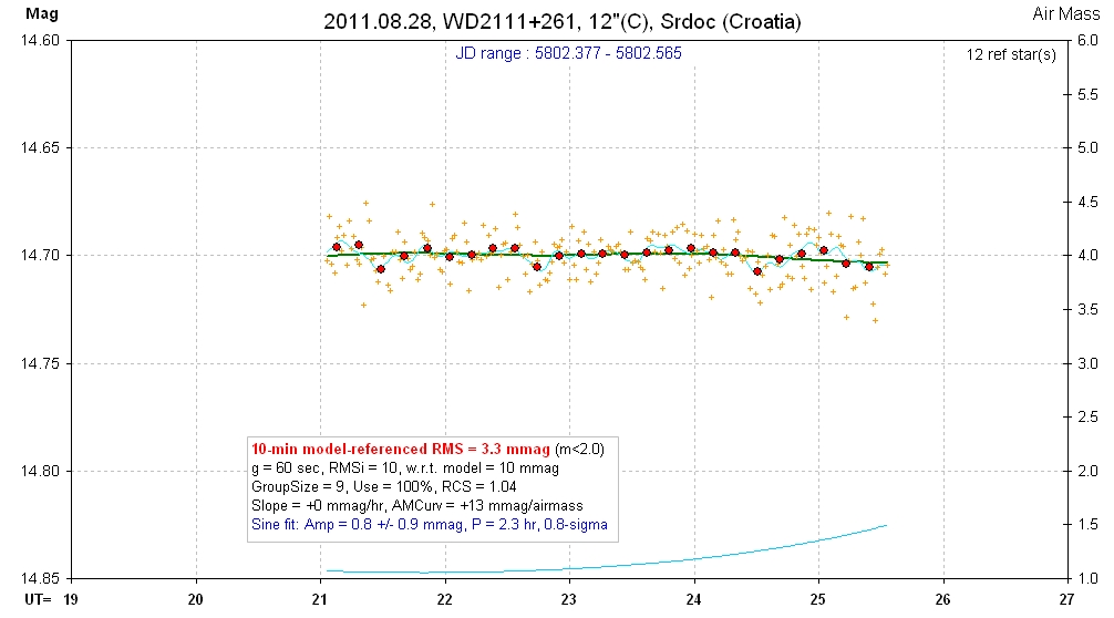
Same data as above, but expanded mag scale for showing sinusoial fit.
______________________________________________________________________________________________________________________________
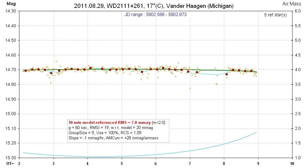
raw spo Numerous high clouds that occasionally obstructed view. Even though I don't see variability inthis LC I show a solution for it below.
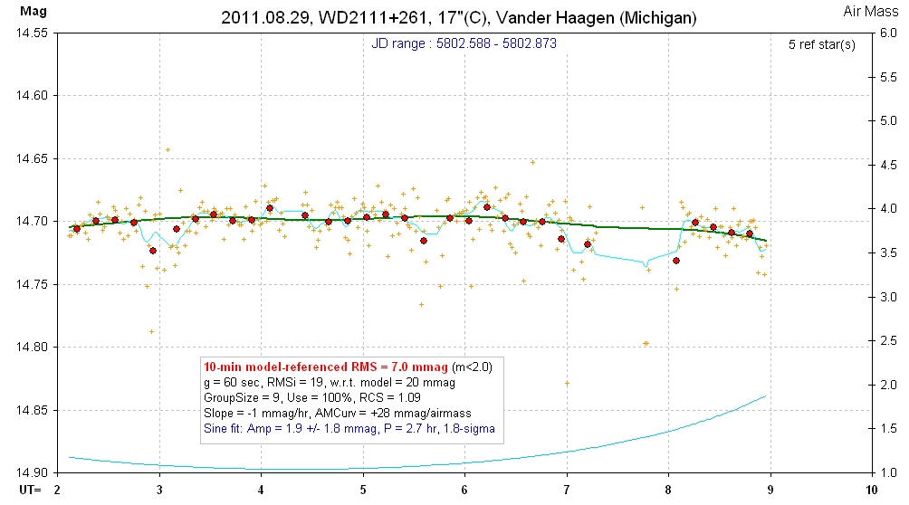
Same data as above, but expanded mag scale for showing sinusoial fit.
______________________________________________________________________________________________________________________________
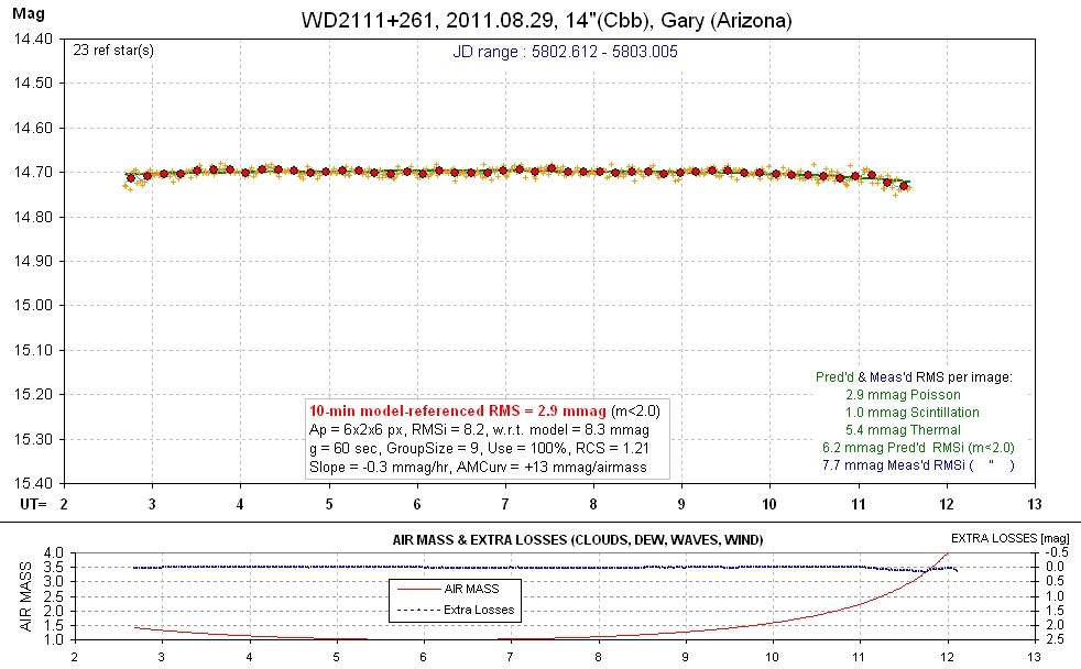
raw spo For an expanded mag scale version of this LC, see below.
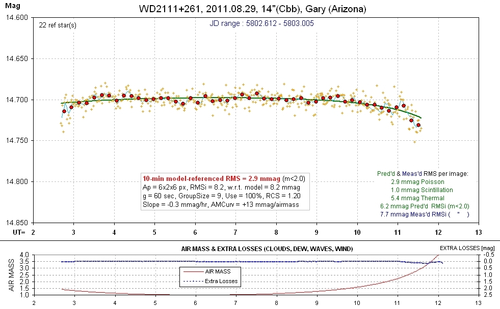
I don't se any sinusoidal variation in this LC, but if you want one see what a formal solution gives, below two plots.
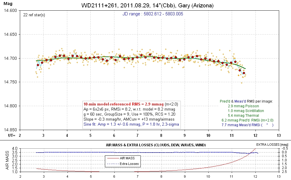
Same data as above, but showing solution when starting near a short period local minimum (1.8 hr). I don't believe this sinusoidal variation.
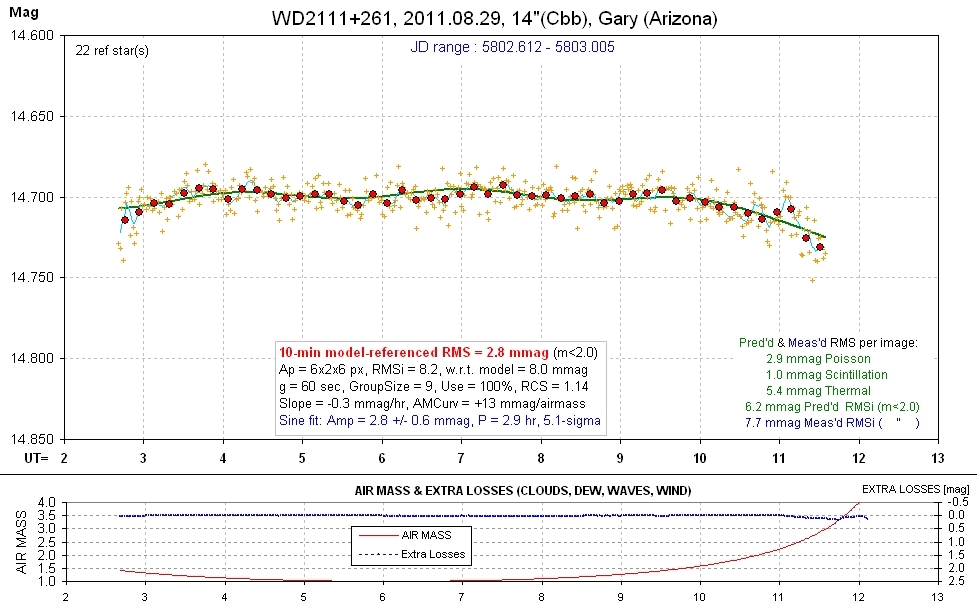
Same data as above, but starting the solution near a local minimum with a longer period. This has a greater statistical significance than the short period.
______________________________________________________________________________________________________________________________
raw spo To see the small sinusoidal variation look at next plot, below.
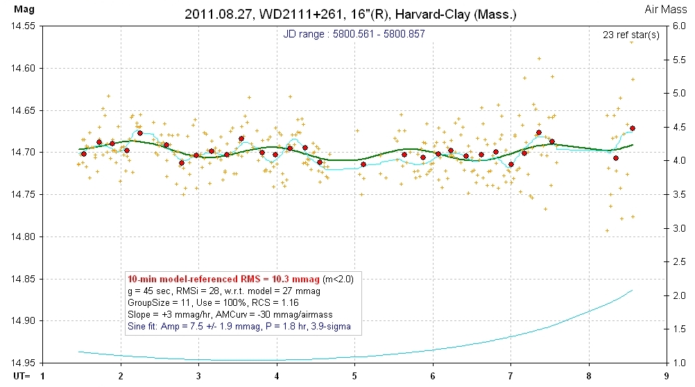
Not very impressive, but statistically significant (3.9-sigma), and consistent with solution for other LCs.
______________________________________________________________________________________________________________________________
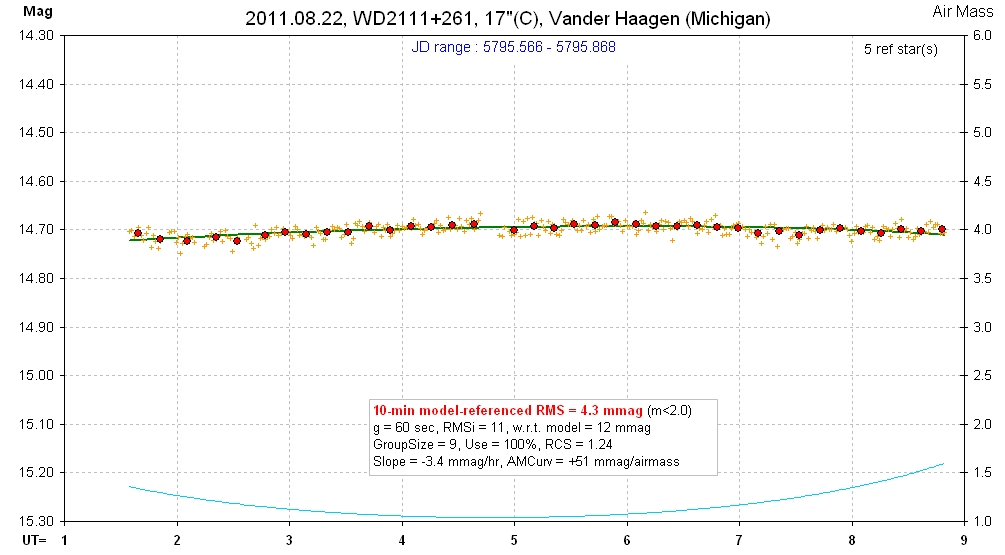
raw spo
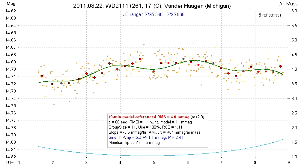
Same data as above, but zoomed mag scale, showing a statistically significant sinusoidal variation (4.8-sigma).
______________________________________________________________________________________________________________________________
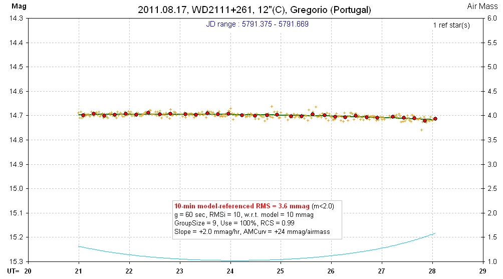
raw spo There's a very small amplitude sinusoid variation, seen a little more clearly in the next LC plot, below.
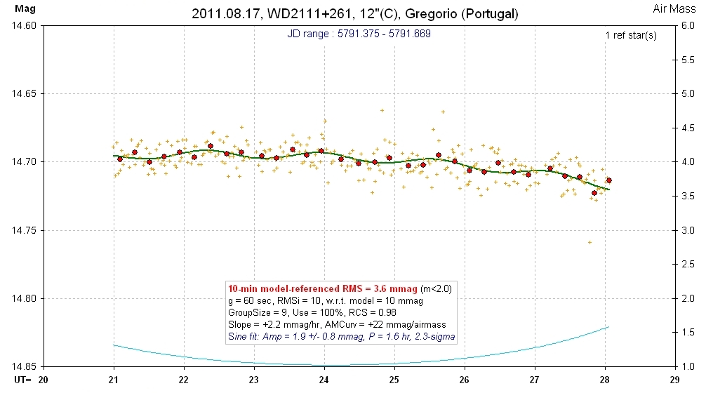
Only a 2.3-sigma result.
______________________________________________________________________________________________________________________________
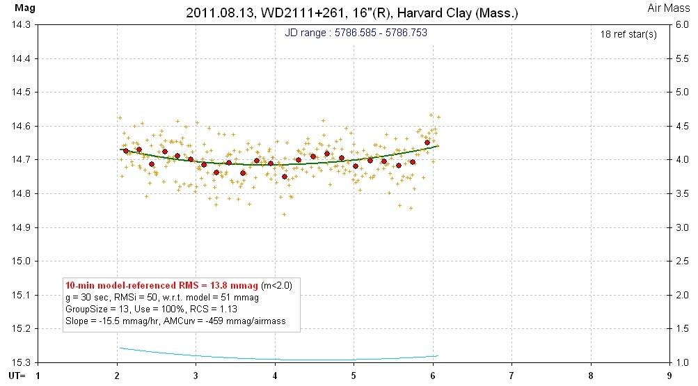
raw spo This LC looks too noisy for solving for a sinusoidal variation, but let's try; see below.
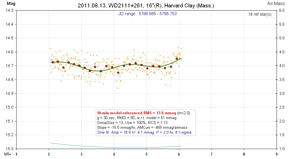
Same data as above, but with sinusoid fit (which is technically statistically significant at the 4.1-sigma level).
______________________________________________________________________________________________________________________________
raw spo See LC below for mag zoom.
Same data as above, but mag scale zoomed to show siusoid fit.
______________________________________________________________________________________________________________________________
raw spo See LC below for mag zoom version.
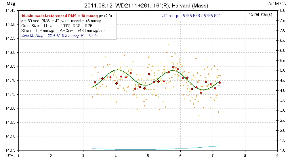
Same data as above, showing sinusoid fit. Note that if this variation is real it has an amplitude 5 to 10 times greater than all other LCs for this object in this archive. Since this is the noisiest LC we should be suspicious of it having the largest amplitude. In other words, when there's a pattern of variation amplitude being proportional to LC noise level, as appears to be the case for this object, we should be wary of all apparent amplitudes.
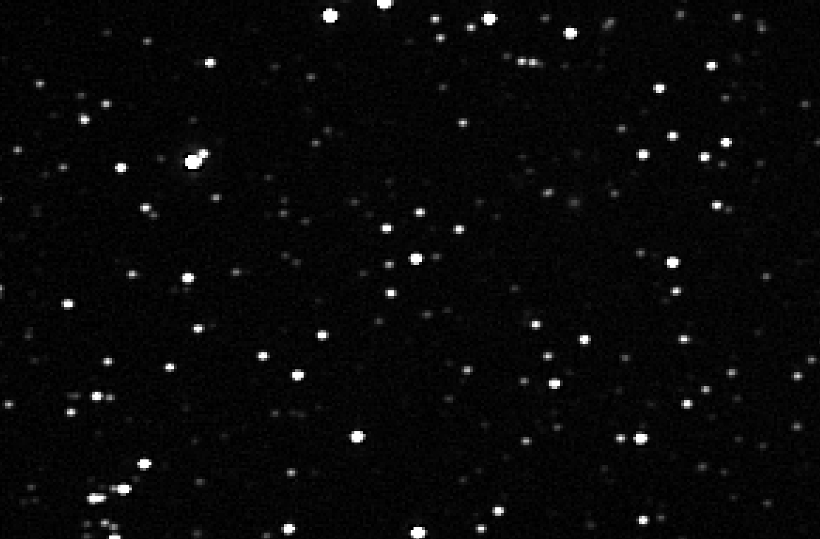
Finder Images
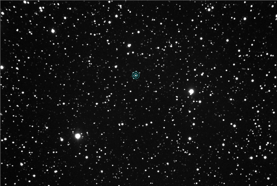
FOV = 27 x 18 'arc, north up, east left. FWHM ~ 3.0 "arc. 5-minute toal exposure time.
Zoom of above image.

Aladin image.