So far we've assumed that the emitting region is a half-space with uniform temperature throughout. This assumption can be violated in two ways: 1) physical temperature can vary with viewing angle withint the antenna pattern, and 2) physical temperature can vary with depth along the line-of-sight for a specific view. Each of these wil be treated in this chapter.
Angular non-uniformity is a trivial case to treat. If, for example, half of an antenna pattern projects onto a surface with physical temperature T1 and the other half projects onto a surface with physical temperature T2, then since the rate of photon emission is linearly proportional to physical temperature (as described in Chapter 1) we know that the apparent brightness temperature of the two materials viewed simultaneously by one antenna beam will be the average of T1 and T2.
Depth non-uniformity is more difficult to understand.
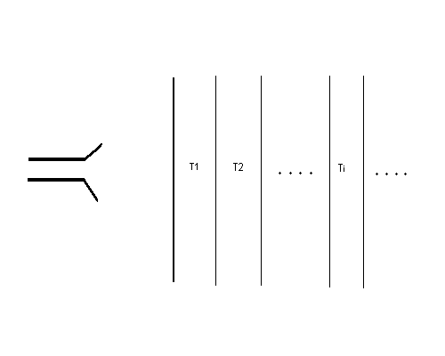
Figure 4.1 This diagram of a emissive material in a half-space with designated layers 1 to infinity will be used in the text to explain the radiative transfer equation. Photons emitted from layers at temperature T1, T2, etc. are received by a horn antenna and radiometer on the left.
First we'll treat the general case in which temperature varies with depth in a manner that is not restricted to linear. The temperature at layer "i" is Ti, and "i" goes from 1 to infinity (throughout the half-space). The photons from layer 1 that leave the surface in a direction toward the horn antenna travel without intervening absorption all the way to the horn, where they are "captured" and delivered to a detector in a radiometer. The thickness of layer 1, and all other layers, is chosen small enough that the layer is almost transparent. The probability that a photon incident upon layer 1 will be absorbed is f1, so the probability of a photon traveling though the layer without being absorbed is 1-f1. The number of photons emitted by layer 1 is only f1 times what would be emitted by a thick blackbody at temperature T1. (That's intuitive, and I won't try to prove it.) Therefore, the number of photons from layer 1 that are received by the horn antenna is proportioanl to T1 * f1.
The number of photons emitted by layer 2 will be proportional to T2 and f2. The fraction of them that pass through layer 1 is 1-f1. So the layer 2 contribution to the number of photons received by the horn antenna is proportional to T2 * f2 * (1-f1). A pattern is emerging, described by the following equation.
TB = T1 * f1 + T2 * f2 * (1-f1) + ... + Ti * f i * (1-f1) * (1-f2) * ... * (1-fi-1) + ...
If we double the thickness of a layer then f will double, so let's say that f = K * w, where K is an absorption coefficient and "w" is a thickness. For a given layer, we have fi = Ki * wi. The number of photons emitted by a layer is proportional to its temperature, and is also proportional to its absorption coefficient and thickness, so this number is proportional to Ti * K i * w i . It's not necessary that all layers be the same thickness, only that they have a transparency close to 1 (so that this model will be correct in the limit of ever shallower layers).
This model for radiative transfer is straightforward, and can be easily programmed. A radiative transfer model using integrals follows from this layer model. Let's adopt the following terminology:
T(r) = source function (temperature versus range from the observer),
W(r) = weighting function (proportional contribution versus range from the observer),
TB = observed quantity (same units as T),
then TB can be expressed using integrals, where instead of discrete layers we employ the independent variable r (range).
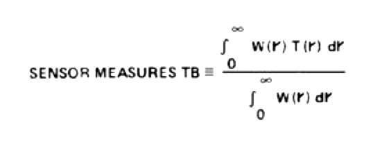
Figure 4.2 Integral expression for what a radiometer measures when the source function (temperature) varies with range, as in T(r), and a weighting function varies with range, as in W(r).
Let's consider a simple case in which Ki is the same for all layers, or using the integral equation notation K(r) is a constant. Those experienced with integrals will notice that for this case the weighting function W(r) becomes a simple exponential function having the following form:
W(r) = e-r/constant
It may also be obvious to those experienced with exponentials that an exponential weighting function applied to a linear source function produces a result that is the same as the source function at the location where the weighting function has the value 1/e. The constant in the above equation is referred to in the remote sensing community by the term "applicable range" - for obvious reasons. If the reader is unsure of this, then please consider a proof of this to be a "homework assignment."
This meaning for "applicable range" is very important for those using an MTP. What it says is that if we assume that temperature changes linearly with range throughout an emitting material, and if we can further assume that the absorption coefficient of the emitting material is the same throughout the relevant part of the line-of-sight path into the emitting material, then the brightness temperature measured by the MTP is equal to the temperature at a range given by the "applicable range."
In Fig. 4.1 it was assumed that there was a vacuum between the horn antenna and the first layer, but now it is time to bring that first layer right up to the horn antenna. This is the situation for observations with an MTP embedded within the emitting material, the atmosphere.
Now that the reader is imagining an MTP flying within the atmosphere, let us further imagine that the MTP horn antenna is rotated so that it views the atmospheric emission at an angle inclined "theta" degrees above to the local horizon, as depicted in the following figure.
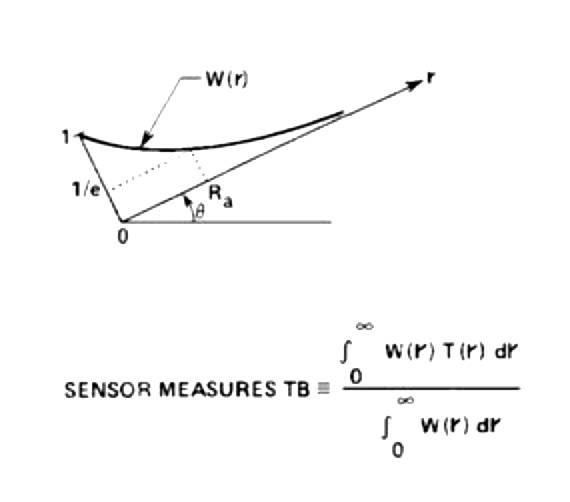
Figure 4.3. Geometry of an MTP looking in a direction inclined above the horizon and measuring a brightness temperature, TB, that is approximately equal to the atmosphere's temperature at an applicable range Ra.
The MTP's measurement of brightness temperature can be used to estimate the temperature at the location of the applicable range Ra, provided the applicable range can be calculated from the atmosphere's absorption coefficient using the relation Ra [km] = 1/K [km-1], where K is the atmosphere's absorption coefficient [Nepers/km] at flight altitude. Notice that from simple geometry that the physical temperature inferred from a brightness temperature measurement can be assigned to an altitude relative to the altitude of the MTP instrument. This leads to the concept of "applicable altitude," Za. With the MTP mounted in an airplane flying at the altitude Zo,
Za = Zo + Ra * sine (theta)
Provided T(z) is a linear function (along the line-of-sight), it is straight forward to convert TB(theta) to T(z). This insight provides a glimpse of the basic remote sensing strategies that will be explained in more detail in future chapters. Before this is done, however, we should have a better understanding of the absorption coefficient of the atmosphere, which will be treated in the next chapter.
Note: It is not my intent to dwell on the details of the radiative transfer equation since it is part of a well-established scientific literature. The reader may want to confirm some statements made in the previous paragraphs by doing self-assigned homework. I hope this is not necessary, as there is much material to cover in future chapters, and I don't want to review at every instance what is well-known within the remote sensing community. My intent is to describe things that are somewhat unique to the MTP. The goal of this chapter was to show that when temperature varies with range, MTP observes a brightness temperature that is approximately the same as the physical temperature at a range called the "applicable range" - which can be easily converted to an altitude using simple geometry.
Go to Chapter #5 (next chapter)
This is Chapter 4
Go to Chapter #3 (previous chapter)
Return to Introduction
____________________________________________________________________