ER911014 CAT EVENT
Overview of Flight ER911014
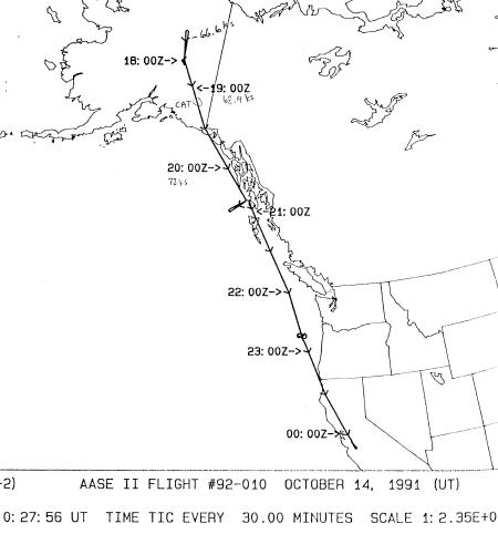
The flight of October 14, 1991 was a ferry flight from Fairbanks, AK to Moffett Field, CA.
Figure 1. Ground track of flight ER911014. The CAT encounter occurred over southern Alaska.
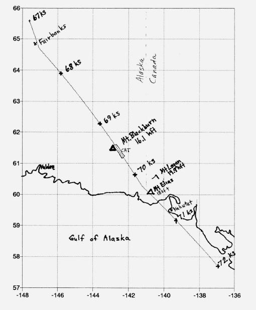
Figure 2. Close-up of ground track showing location of CAT encounter in relation to mountains
The region of interest for this report is southeastern Alaska, which is shown in the expanded map in Fig 2. The moderate CAT patch occurs in association with 16,000-foot Mt. Blackburn. Thus, the CAT is probably produced by mountain waves interacting with a pre-existing layer of high wind shear. Whereas the ER-2 is flying a heading of 148 degrees, the wind is out of the SSW (toward an azimuth of 33 degrees); thus, the ER-2 is flying 115 degrees away from the wind direction.
Isentrope Altitude Cross-Section
The next figure is a curtain cross-section of isentrope surface pressure altitudes. It was constructed from data taken by JPL's Microwave Temperature Profiler mounted in one of NASA's ER-2 aircraft, hereafter referred to as the MTP. The "jumbled" region from 69 to 70 ks (kilo-seconds) is a mountain wave. Figure 4 is a "zoomed" version of the mountain wave part of the previous isentrope altitude cross-section (IAC). The peak-to-peak vertical excursions of some isentrope surfaces is over 1000 meters. The isentrope pattern of vertical displacements exhibit horizontal wavelengths that range from 125 to 580 seconds, or 26 km to 120 km.
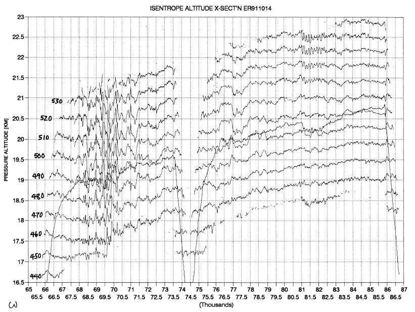
Figure 3. Isentrope altitude cross-section, showing the large displacements early in the flight (at about 69 to 70 ks).
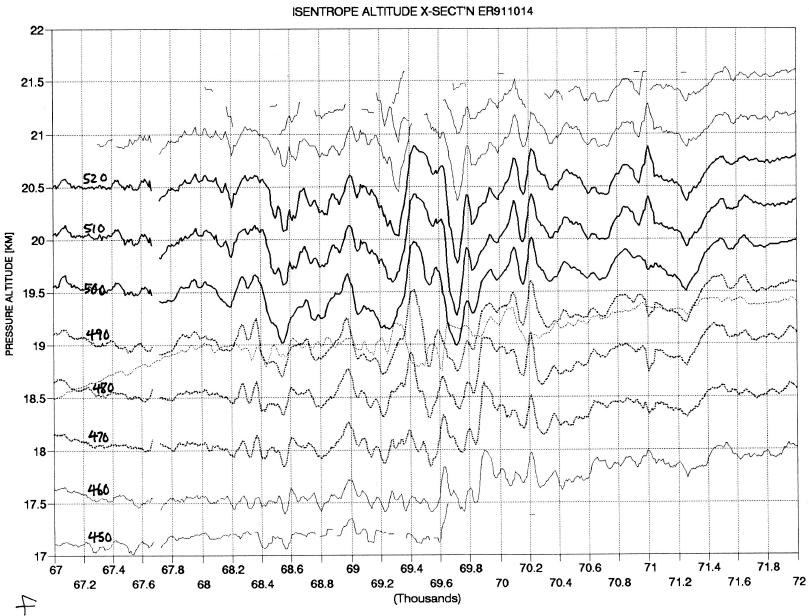
Figure 4. Zoom of mountain wave region of previous figure.
Figure 5 zooms the previous IAC further, and shows the region of greatest isentrope altitude displacement. The flight path is shown by the thin "dotted" line. The vertical "hatching" on the flight path line shows where the MTP's vertical accelerometer exhibited large excursions in response to turbulence. The pilot, Jim Barrileaux, reported "moderate CAT about 200 miles east of Anchorage." He also reported encountering large temperature excursions, and he disabled the "auto-Mach hold" in order to fly the airplane manually.
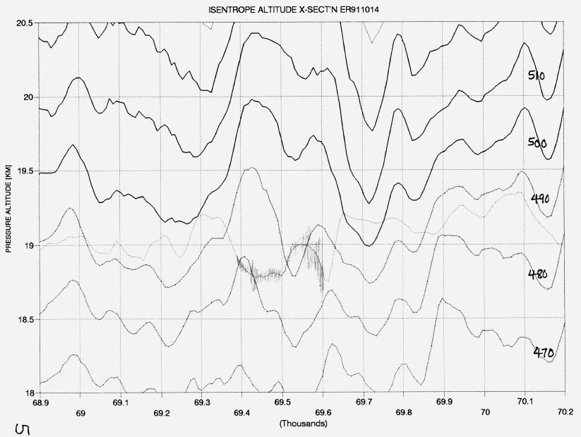
Figure 5. An even closer zoom view of the previous figure, showing where turbulence was encountered (hashy structure along aircraft flight path).
Vertical Accelerometer Data
The upper panel in Figure 6 is a trace of the MTP's vertical accelerometer (a separate sensor from the aircraft instrumentation). Readings are made at a rate of approximately 2.5 Hz. The accelerometer output is low-pass filtered at 20 Hz (half-response) before readings are made, so the readings are an under-sampled representation of the actual aircraft motion. The under-sampling is only a shortcoming when attempting to derive CAT intensity, as non-CAT flight does not contain significant vertical motions that require sampling at intervals less than 0.4 seconds. An empirical correction for our under-sampling of the sensor has been established, so the data actually can be used to quantify CAT intensity.
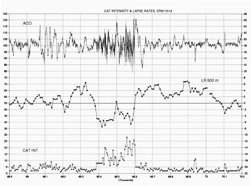
Figure 6. Vertical accelerometer (upper tace), lapse rate for a 500-meter thick layer centered on aircraft altitude (middle trace) and CAT intensity (lower trace).
The upper trace has two behaviors of note: KH waves, and CAT.
At 69.1 to 69.2 ks there are sinusoidal vertical motions with amplitude
0.25 g-units and a
characteristic period of 19 seconds, or 4.0 km. I identify these to
be Kelvin-Helmholtz waves, which are produced when vertical wind shear
"overturning forces"
approach the temperature field's "restoring forces." KH waves
grow in amplitude when the temperature field has insufficient vertical
static stability to suppress vertical motions. Such waves usually occur
in layers with high values of vertical wind shear and lapse rate.
A "rule of thumb" states that the horizontal wavelength of KH waves is
approximately 7 times the layer's thickness. Accordingly, the 4.0 km wavelength
"predicts" the presence of a 600 meter thick layer containing high wind
shear and lapse rate. (More about this region later.)
The trace at the bottom, labelled "CAT INT," is the "5-second maximum of 1-second peak-to-peak of the accelerometer readings." Since during CAT there is some "energy" at vertical motion frequencies higher than can be sampled by 2.5 Hz readings (but lower than about 15 Hz), the "CAT INT" lower trace will under-represent peak-to-peak excursions during periods of CAT. I estimate that when CAT is present the CAT INT trace should be multiplied by 1.3. Thus, whereas the CAT INT trace reaches a maximum of 0.28 g-units (at 69.55 ks), a more frequent sampled version of our accelerometer output might have produced a CAT INT value of approximately 0.36 g-units. This is generally considered to be within the range of "moderate" CAT.

Figure 6a. Zoomed version of previous figure, showing each 9-second cycle's lapse rate measurment. The green star symbols on the green dT/dZ trace are the individual MTP data cycle measurements of dT/dZ.
In Fig. 6a, at 69.6 ks, the lapse rate changes from -6 [K/km] to +3 [K/km] in just two 9-second data cycles! This corresponds to a distance flown of 3.8 km. Considering that the "look distance" is defined by an exponential function having a 1/e distance of about 1.8 km (at this altitude), the appearance of a 3.8-km transition means that the actual transition was approximately 3.3 km. The other transition, from 69.345 to 69.40 ks, is more gradual, being 11.5 km long.

Figure 6b. Expanded scale of the "CAT exit region" of the previous figure. The thin black trace is what the MTP would measure if dT/dZ changed abruptly at 69605 ks from -6.1 to +3.6 [K/km], the thick red dotted trace is what MTP would measure with a 2-km wide linear transition, and so forth, as shown in the legend.
This figure shows that the dT/dZ change from -6 to +3 [K/km] was approximately 2 km wide. Recall that the MTP measurements are a weighted average of true air temperature ahead of the aircraft, and the weighting function (at this altitude) is an exponential with a 1.8 km 1/e distance. Thus, if lapse rate changed abruptly, the MTP would measure a "soft" lapse rate transition. The thin black trace in Fig. 6b is what MTP would have measured if dT/dZ changed abruptly from -5.9 to +3.1 [K/km] at 69605 ks. If the LR change occurred with a 2-km transition, for example, MTP would have measured the thick black dotted trace in the figure. The thick continuous blue trace corresponds to a 4-km linear transition, and it exhibits a noticeably poorer fit to the measurements. The statistically best fit has a linear transition width of 1.4 +/- 0.5 km.

Figure 6c. RMS of simulated "dT/dZ versus time" series versus width of dT/dZ transition region. The best fit occurs for a transition width of 1.37 +/- 0.40 km.
Figure 6c provides a solution for the width of the lapse rate transition width, and it is 1.4 +/- 0.4 km. The standard error just cited is a formal statistical result, and does not allow for uncertainties related to subjective parts of the procedure leading to the solutions under evaluation. For example, referring to Fig. 6b, I arbitrarily forced all solutions to have dT/dZ = +3.6 [K/km] after passing out of the CAT patch. Also, I used adjusted two other parameters for optimum fit - a time offset paramter and the dT/dZ asymptote value for within CAT (approximately -6.1 [K/km]). Taking these factors into account, I will apply a subjective correction to the formal SE and state that it is my position that the width of the lapse rate transition layer was 1.4 +/- 0.8 km. This distance is travelled by the ER-2 in 6.7 +/- 4.0 seconds. I don't know if this is in agreement with theory, but it might provide a constraint on models.
One additional qualification to the foregoing must be made. The value for dT/dZ within the CAT patch, approximately -6.1 [K/km], is probably too high! If the CAT patch had dT/dZ = -9.7 [K/km], for example, and if the CAT was confined to a layer that was 1 km thick (see below), and if the ER-2 were flying in the middle of the layer (as shown, below), then the MTP measurements would be approximately -7 or -8 [K/km] due to the fact that each measurement has a weighting function with an e-folding distance of 1.8 km. For example, when the MTP views upward 10 degrees from the horizon, approximately 20% of the weighting function will be beyond the top of the adiabatic layer at 0.5 km above flight level. This will reduce the "measured" dT/dZ from a true value of -9.7 [K/km] to approximately -7.8 [K/km] (if the layer above is isothermal). Therefore, we should consider that the actual dT/dZ at flight level might have been close to adiabatic while flying within the CAT layer, whereas it only appeared to be -6.1 [K/km] due to the shallowness of the layer. The point to be emphasized here, though, is not what dT/dZ value existed within the CAT layer; rather, whatever the value was for dT/dZ within the CAT layer it abruptly changed to a "compression" value outside the CAT region, and the transition occurred in approximately 1.4 km of horizontal distance.
Figure 7 shows a longer interval of accelerometer data. Light CAT is generally considered to begin for peak-to-peak motions of about 0.10 g-units. Allowing for the correction factor of 1.3, which should be applied to this data when CAT exists, we can place our threshold for light CAT at 0.07 gunits. Thus, there are light CAT encounters at 68.4 ks and 70.2 ks. The event at 69.92 ks appears to be an updraft, according to the upper trace, and should not be considered CAT. The slight feature at 69.1 ks can also be disregarded because it as an artifact of the CAT INT algorithm in the presence of large amplitude (non turbulent) waves.
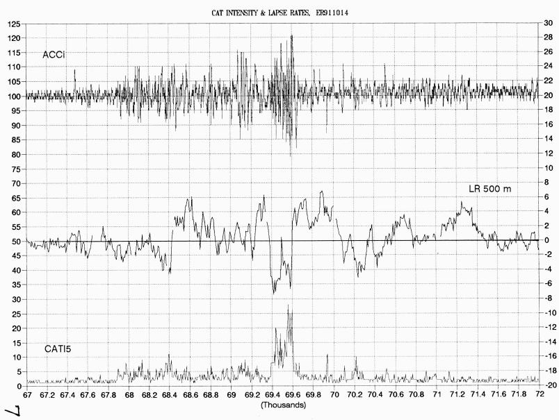
Figure 7. Same as previous figure except a larger span of time is shown.
Lapse Rate
The middle traces in Fig.7 is MTP measured lapse rate, LR (defined here as the vertical gradient of temperature), for a layer 500 meters thick. Referring to Fig. 7, the LR is generally isothermal (0 K/km), as is usually the case in the lower stratosphere. However, there is a 600 km region, from 68.4 to 71.4 ks, that includes high LR values. It is quite rare to encounter LR as high as + 5 K/km at these altitudes, yet within this region such high values occur several times.
It is also unusual to encounter layers with LR as low as -5 K/km, yet such a region occurs at 69.4 to 69.6 ks, surrounded, ironically, by high LR air. But the greater irony, and of course this is a meaningful clue to what is physically going on in this region, is that the very low LR air is located precisely with the moderate CAT patch. This can be seen better in Fig. 6. There is an almost perfect one-to-one correlation between CAT intensity and LR. Note the abrupt ending of CAT at 69.6 ks, and the correlated abrupt LR transition from low LR to high values. Note also the brief reduction of CAT intensity in the middle of the patch (at 69.5 ks) and the correlated brief rise in LR value.
Which is cause and which is effect? CAT must cause the negative change in LR, as a complete mixing of air parcels in a region will necessarily produce adiabatic LR values (-10 K/km). In going from +5 K/km to -7 K/km at the max-CAT time, the LR went approximately 80% of the way from its pre-CAT value (assumed, here, to be + 5 K/km) to the adiabatic value that a complete mixing would produce. Thus, the volume of air that was mature turbulence must have occupied at least 80% of the air volume sampled by the MTP instrument. If the layer of CAT was limited to 600 meters thickness, and if this layer had a true LR of -10 K/km, then we can account for the measured LR by speculating that 20% of the MTP "antenna reception field" lay beyond the CAT layer. Given the geometry of this situation, this 20% value is possible. I conclude that the low LR parts of maximum CAT intensity (at 69.44 and 69.55 to 69.6 ks) may have in fact produced an adiabatic LR.
Referring to Fig. 7, it is apparent that LR also goes negative at the times of the two light CAT encounters, at 68.4 and 70.2 ks. This light CAT produced LR values of -4 K/km versus the -6 or -7 K/km during moderate CAT.
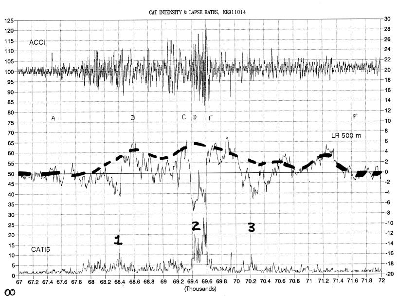
Figure 8. Suggested pre-CAT lapse rate trace (middle) for encounters 1, 2 and 3. Events "A" through "F" are identified here.
It will be instructive to imagine what the LR trace would have looked like before the CAT altered it. Figure 8 is an attempt to do this. In drawing the thick dashed line I was guided by the assumption that the greater the CAT the greater is the negative change in LR. Thus, starting at 67.85, when "very light" CAT begins, the dashed line is slightly higher than the measured LR trace. At the light CAT event "1" the LR dip is considered accounted for by continuing the dashed line upward. Higher than measured values are sustained between "1" and "2" because very light CAT is present throughout this region. The light CAT event "3" is allowed for in the same manner as for event "1." What emerges is a large, synoptic scale region of elevated LR, extending from about 68.0 ks to 71.5 ks. This region is 1.0 hour in extent, or 750 km.
These data further support my suggestion (Gary, 1991) that on a mesoscale LR is negatively correlated with CAT, whereas on a synoptic scale LR is positively correlated with CAT!
I would like to present a synoptic scale picture of what might be happening,
for what it's worth (only qualfied meteorologists are allowed to snicker
here). I picture a synoptic scale air mass over-riding another, and
the interface between them is slightly sloped. The interface "layer"
contains transitions in both wind vector and temperature. The dynamics
of the one air mass "sliding off" the other causes a thinning of the interface
layer, analogous to losing "lubricant" between two solid objects with flat,
sloped surfaces at their interface (it's obvious that I've never had a
meteorology course). The isentrope surfaces come together, as if
under compression, and the isotach surfaces do the same. The interface
layer has more closely spaced isentropes, creating an inversion layer.
Synoptic scale processes continue to compress the interface region, bringing
isentrope and isotach surfaces together. I believe this is the scenario
for the ER-2 flight under discussion, and by good luck the ER-2 was flying
within the transition layer for 1 hour. The existence of a mountain
beneath the middle of this synoptic scale region of compression was another
stroke of good luck, as it provided an additional distortion that brought
isentrope and isotach surfaces together with the result that Richardson
Number decreased an additional amount
that was sufficient to trigger CAT.
Altitude Temperature Profiles
In Fig. 8 the symbols "A" through "F" indicate times for which "altitude temperature profiles" have been constructed. The profiles are presented in Figures 9A through 9F.
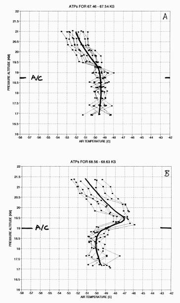
Figure 9A and 9B. Altitude temperature profiles, T(z), from the MTP instrument. Each thin trace with small square symbols is an individual 14-second measurement, while the thick trace is an average of the group. Aircraft altitude is indicated by the "A/C" symbol. The first profile group is "normal" or "undisturbed." The second group exhibits a dramatically rapid vertical compression, creating an inversion layer due to adiabatic heating.
Figure 9A is "normal" in the sense that no inversion layer temperature structure is present. The lapse rate is indeed isothermal at flight level (18.75 km), which is consistent with the LR trace in Fig. 8. Figure 9B shows the presence of a strong and shallow inversion layer at flight level, FL. Note that the inversion layer is about 500 meters thick, and that compression is a likely origin due to the fact that the two profiles are identical below FL but warmer than in Fig. 9A above FL. The maximum temperature difference is 3 K (at 19.5 km), implying a vertical descent (compression) of 300 meters.
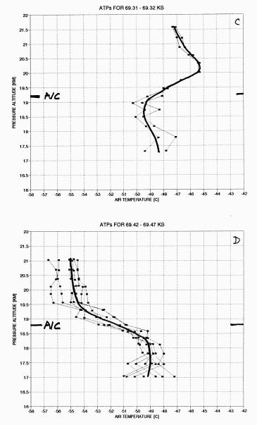
Figure 9C and 9D. This pair of T(z) groups are from "just before" to "within" a CAT patch. Notice how the mixing of air by CAT motions has converted an inversion layer into an almost adiabatic layer.
Figure 9C is immediately before the moderate CAT event, and this profile shows the maximum amount of "warming." The air at 20 km is 5.7 K warmer than the air at the same altitude in Fig. 9A. This could be interpreted as a 570 meter descent if it can be assumed that the air at location "C" originally had the same temperature profile as in "A." Note that the inversion layer is 1000 meters thick at "C."
Figure 9D is for a time only 2 minutes after the profile in the previous panel. At 20 km the air is 9.5 K cooler at "D" than at "C"! The air below FL is unchanged. If it is assumed, for the moment, that mountain waves were not moving air up and down in a non-mixing, reversible process, then by overlaying panels 9C and 9D, and drawing adiabat lines between the two profiles, it is possible to account for the colder temperatures at 20 km by hypothesizing that the redistribution of air produced by turbulence caused air that originally was at 19.4 km to end up at 20 km. Continuing with this assumption that mountain waves are not present, the turbulence redistribution would have to extend from 18.5 km to higher than 22 km. This strikes me as a tremendously thick layer for CAT, and shows that it is necessary to allow for the mountain wave motion before calculating altitude redistribution statistics.
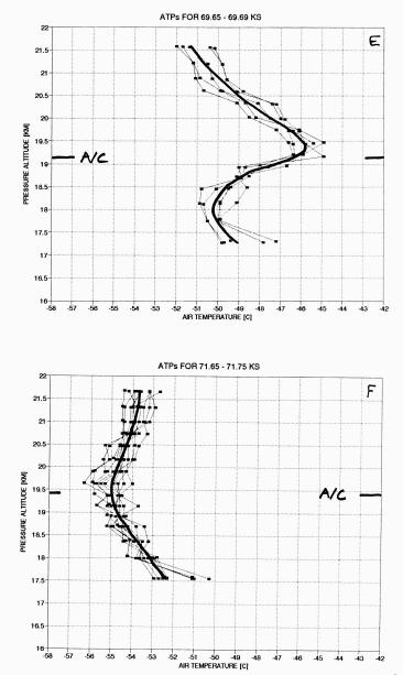
Figure 9E and 9F. Another illustration of the temperature field immediately outside a CAT patch (upper) and a distant location apparently not undergoing vertical compression by synoptic scale forces.
Figure 9E is for a time immediately after the abrupt cessation of CAT. An inversion layer is present which is somewhat similar to the pre-CAT inversion layer in Fig. 9C. Inversion layer thickness is about 1000 meters, but the altitude of the layer is about 800 meters lower at "E" compared to "C." The aircraft went from flying near inversion layer base, at "C," to flying near inversion layer top, 6 minutes later at "E." These comparisons support the notion that the interface (compression) region is sloped. Figure 9F is for "normal" air, and shows that beyond the 600 km "compressed" region, from 68.4 to 71.4 ks, inversion layer structures are not present.
For anyone wishing to view more T(z) detail during the pre-CAT through post-CAT period 69 to 70 ks, click ATP Details.
Old RRi Analysis
In my original analysis of this flight I used the "sinle regression" (SR) method for determining vertical wind shear, VWS. This led to a RRi(t) given in the next figure.
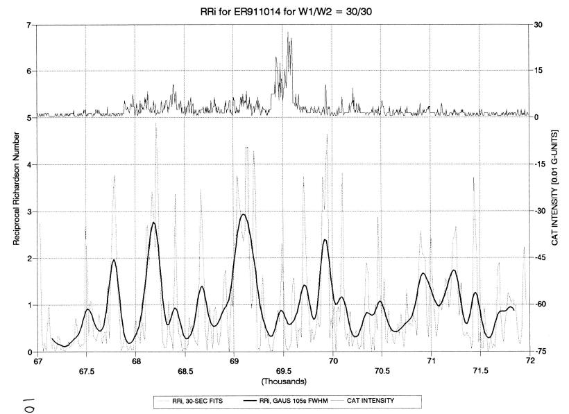
Figure 10. Reciprocal Richardson Number, RRi, derived using a "single regression" method for deriving vertical wind shear, VWS. I suggested that the CAT patch at 69.5 ks was surrounded by a region of higher than normal RRi.
Using a warning threshold of 2.0 for RRi derived using the SR method, and adopting the 105-second Gaussian average trace, would produce warnings of 19.8 minutes flying forward, and 4.8 minutes flying "backwards." RRi goes low during CAT, as it should theoretically.
New RRi Analysis
The rest of this web page will consist of new analyses of VWS and RRi, using the DD method (Difference Data method) for inferring VWS.
Using a difference time of 10 seconds to determine VWS, then calculating RRi, produces the following figure.

Figure 11. RRi and accelerometer peak-to-peak for a 1.4-hour portion of flight centered on the "moderate" CAT encounter. The thick black trace is a 2-minute average of RRi, plotted at the centroid of the data producing the RRi value. Shifts of 1-minute are required to produce a simulated trace of "RRi based only on data in hand" for determining warning times. The "warning" indication at 70.4 ks corresponds to "backwards" flight.
This trace of DD-based RRi is approximately the same as the SR-based RRi trace in Fig. 10. The major difference is the presence of a high DD-based RRi feature at the time of maximum CAT. I suspect that this is not real, and is an artifact caused by the DD-method's susceptibility to horizontal wind gradients during the calculation of VWS. This is pure speculation, and is based on the desire to reconcile measurements with theory.
Warning Times
Warnings with "data in hand" would begin at 68.2 ks, or 19.8 minutes
before the first CAT exceeding 0.2 g-units (this is based on shifting the
thick black trace 1-minute's worth to the left). Flying "backwards"
(i.e., shifting the thick black trace to the right 1 minute's worth) yields
a warning time of 12.3 minutes to the most intense CAT. These warning
times assume an RRi warning threshold of 2.5, as adopted for the previous
flights. I admit to feeling uneasy about claiming a warning time
as large as 19.8 minutes, since such a long lead time could qualify the
warning as a false alarm. However, if an instrument were flying in
the cockpit it would have started issuing warnings 19.8 minutes before
encounter, and would have continued to issue warnings until the encounter
occurred (since the RRi > 2.5 threshold was exceeded frequently during
the 19.8 minutes preceding the encounter).
| Flight Direction | CAT Onset | Warning Time |
| Forward | 69.4 ks | 19.8 minutes |
| Backward | 69.6 ks | 12.3 minutes |
As with the other flights, I shall defer analysis and discussion of false alarms until I perform a systematic analysis of a selection of pilot-reported smooth flights.
Conclusion
The present flight provides a clear case of mountain wave generated CAT. The lapse rate record shows that vertical compression occurred immediately before CAT onset, and immediately following CAT cessation. The RRi derivation also supports the idea that vertical compression caused RRi to increase and CAT to occur. Hence, this flight data provides strong support to the hypothesis that CAT is generated as a result of vertical compression.
This flight data has allowed what may be a "first-ever" determination of the horizontal width of the lapse rate transition region at the edge of a CAT patch. It was found that dT/dZ changed from a value more adiabatic than -6.1 [K/km] within a CAT patch to +3.6 [K/km] outside during a 1.4 +/- 0.8 km transition region.
Return to Home Page of this web site.
____________________________________________________________________
This site opened: August 26, 2000. Last Update: September 23, 2000