Bruce L. Gary (GBL)
ABSTRACT
This web page is devoted to my analysis of observations of the 2003 UV Persei superoutburst "superhumps." My observations are described first, as well as those of Arto Oksanen and other AAVSO members.INTRODUCTIONSuperhumps (brightenings of ~0.2 magnitude) occurred at intervals of approximately 95.8 minutes, but there were large departures of peak brightness times from a constant period model. If the timings of the superhump peaks are converted to periods then the apparent period varies from ~95.45 minutes to ~96.2 minutes during the first 9 days of the superoutburst.
This web page describes observational results of the cataclysmic variable UV Persei.
Blah, blah, blah.
A description of my hardware and observing procedure is presented in Appendix A.
LINKS INTERNAL TO THIS WEB PAGE
Observations by Bruce L. Gary
Analysis of Arto Oksanen data
Combining Arto Oksanen data with
Bruce L. Gary data
Combining Most of the AAVSO Data
- Longitude Wander Result
Appendix A - Hardware, observing
procedure and analysis procedure
Appendix B - Links to Mv observations
by OAR and GBL
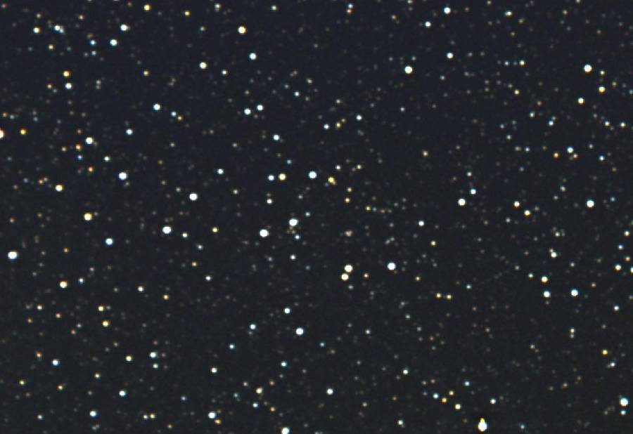
This is a color image of the UV Per region.
Figure 1. UV Per was quiescent (Mv = 16.3) when this color image was taken. The field of view is 58 x 40 'arc, northeast is to the upper-left. The bright stars are saturated in the R, G and B images and so they appear white even though they have a color in unsaturated versions of this image. UV Per (located in the next image) is slightly reddish in a brighter version of this image. [Celestron CGE-1400 (14-inch aperture), Starizona HyperStar prime focus adapter lens, f/1.86, SBIG ST-8XE CCD, SBIG CFW8 and Custom Scientific B, V, and R-filters; MicroTouch focuser, exposures of 6 min, 3 min, and 4 min (BVR), 2004.01.05Z, Hereford, AZ; USA]
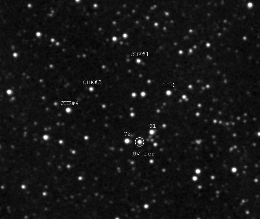
Figure 2. Zoom factor 4, taken when UV Per (circle) was in outburst. The field-of-view is 14.0 X 11.8 'arc (a small portion of the 72x48 'arc full FOV). Star "110" was used as a reference ("comparison") star, and it's magnitude was assumed to be 10.981 (based on Arne Hendon's photometric sequence). The other 5 stars were used as "check stars" to validate internal consistency of the observations. Stars "C1" and "C2" were used by Udalski and Pych (1992) in their study of the 1989 superoutburst. Star "C2" was discovered by Arto Oksanen to be a variable (see below). I have evidence that stars "C1" and "Chk#4" are also variable. Only stars 101, Chk#1 and Chk#3 are constant. [Celestron CGE-1400 (14-inch aperture), Starizona HyperStar prime focus adapter lens, f/1.86, SBIG ST-8XE CCD, SBIG CFW8 and Custom Scientific V-filter; 2003.11.08Z, Hereford, AZ; USA]
Figure 3. UV Per (red) and a check star (green) for a 9.8-hour
observing period on November 8, 2003 UT. The check star is Star "Chk#1"
and appears to be constant, implying that reference star "110" is also
constant.
Figure 4. Check stars C1 and C2 (also referred to as Chk#2 and Chk#5) versus time, assuming reference star "110" is constant. Star C2 variation has an amplitude of 0.031 magnitude (half of peak to peak) and a period of 3.8 hours. A drift was fitted to the data having a value of 0.025 magnitudes per hour. Presumably this is part of a longer sinusoidal variation that merely appears to be linear for the limited observing period.
Figure 5. Star "Chk#3" (green) is constant but the other two have a slight variation. Star "Chk#3" (middle, using right side magnitude scale) has an amplitude of 0.019 magnitude and a period of ~11 hours. The top plot is for "Chk#2" (also called "C1") and it exhibits an amplitude of 0.021 magnitude and a period ~18 hours (this period should be treated with caution).
ANALYSIS OF BRUCE GARY OBSERVATIONS
There are 6 "superhump" cycles in this data set. The interval between maxima for my observations averages 94.68 +/- 0.99 (SE on average) minutes, based on the following table of peak brightness times:
TABLE 1
UT [hr]
are referenced to Nov 8.0
Cy#
UT hrs Interval
1
3.80
2
5.40 1.60 hr (96.2 min)
3
6.95 1.55 hr (92.9 min)
4
8.52 1.57 hr (94.2 min)
5
10.15 1.63 hr (97.8 min)
6
11.69 1.54 hr (92.4 min)
Average period
= 1.578 +/- 0.016 hr (SE on avg)
= 94.68 +/- 0.99 min "
What if we folded the entire data set with a period of 94.68 hours?
Figure 6a. Folded light curve, using a period of 94.68 minutes. A temporal decay of 0.00384 magnitudes per hour was adopted as a normalizing correction. The hand fit endeavors to be a "median fit" (instead of an average fit).
It should be noted that some of the variability in this plot is due to real changes in the shape of different superhump cycles. It seems significant that inflections exist at specific times in the cycle during the rise and decay phases. These occur at about -15% and +28% of a cycle (referenced to the cycle peak time). The peak structure can be fitted adequately by two linear sections with an abrupt inflection at the peak.
Figure 6b. Same folded light curve, except centered on low brightness portion of superhump light curve.
The "bottom" of the superhump light curve appears to be "softer" than at any other time, especially just before the rise phase.
Arto Oksanen is at a great latitude in Finland for observing UV Per, as it transits near his zenith and is always high in the sky. His are the first "comprehensive" observations of the 2003 UV Per superoutburst and are the highest quality in the AAVSO archive.
Figure 7. Arto Oksanen V-magnitude measurements for two nights.
The decay rate in this 2-day plot is evident. It also appears that the superhump amplitude is decreasing with time. The decay rate for the average brightness is +0.129 magnitude/day (or +0.00538 mag/hour). During the one-day interval from November 7.9 to 8.9 the average brightness decreased 11.2%, i.e., from 100% to 88.8% of the starting value. The peak-to-peak magnitude range decreased from 0.259 mag to 0.211 mag during the same one-day interval. In other words, the ratio of peak brightness to minimum brightness changed from 1.27 to 1.21 during this one day interval.
There are 5 peak brightness events, and their times are very well-established.
Instead of calculating an average period from this set of period estimates, a better procedure will be employed for determining the period. The table does not contain all the "period information" in the data. A Fourier analysis will show a strongest spectral component at the frequency corresponding to the best solution period. But since Aaron is doing that, I'll achieve what should be a similar result using a different technique. I'll stack the 5 peaks and derive a "median peak shape." Then I'll perform a RMS deviation versus period offset for each of the 5 peaks. This will provide information about the variability of the timing for peak brightnesses.
First, let's look at the 5 peaks in more detail.
Figure 8a. Detail of the November 7 observations of Arto Oksanen.
Figure 8b. Detail of the November 8 observations of Arto Oksanen, using November 7.0 as a UT hours reference.
Since the shapes of each peak are not perfectly determined, and since the shapes may vary slightly from cycle to cycle, a procedure was used to establish a cycle's overall peak time by searching for peak times for each cycle that provided good overall agreement with the region of a peak. For example, I began with cycle #2, and empirically found what time for cycle #1 afforded a good match to cycle #2. Then I proceded to do the same for cycle #3, using the previous pair of matched light curves as a shape to be matched. After doing this for all cycles the following light curve was obtained.
Figure 9. Folded light curves after shifting each superhump cycle of data. Vertical offsets were applied (without changing the scale for a specific cycle). Cycle #2 was used as a reference to which all other cycles were adjusted for best agreement.
Figure 10. Average of first three cycles, then smoothed. Region near peak is the average of all 5 cycles and smoothed.
The superhump brightness shape in this figure is used in the next stage of analysis as a template for final time adjustments for establishing something I will refer to as "peak brightness time" for a specific cycle. The "peak brightness times" for all 5 cycles are presented in the following table. The intervals between neighboring "peak brightness times" is used to determine a period, also listed in the table.
TABLE 2
UT [hr]
is referenced to Nov 7.0
"Peak
Brightness Neighbor
Time" Period
Cy#
UT [hr] [hr]
1
21.38
2
22.96 1.58 (94.8 min)
3
24.58 1.62 (97.2 min)
4
43.705 1.594 (95.625 min) average during
12 cycle interval
5
45.285 1.58 (94.8 min)
Weighted average
period = 1.5935 +/- 0.0017 hr
= 95.61 +/- 0.10 min "
The following figure is a graphical representation of the period column.
Figure 10. Period of superhump spacing based on neighbor peak time separations. With 5 peaks there are 4 neighbor comparisons, labeled 12 for cycle #1 to cycle #2, etc. The weighted average is shown by the horizontal dashed line.
This table's entries of peak brightness times is a better starting place for extracting period information and period variations than are the neighbor differences in the "Period" column. Partly, this is due to the fact that one of the intervals for deriving a period is 12 cycles while the others are one cycle. Even if they were all one cycle apart the "Period" column is not the best way to extract period information since they are just differences between neighbors and extra period information is contained by the other differences. A procedure is described in the next paragraph that makes the best use of the peak brightness times column.
Imagine for a moment that the period is constant throughout the observing interval. If, in addiiton, the shapes were perfectly measured and each shape was the same, the peak brightness times would form a sequence of times that are multiples of the period plus a constant. We could use the first peak brightness time as a reference time, for example, and shift other peak brightness times by the appropriate number of cycles to see if that agrees with the peak brightness time for the first peak. This assumes that we know the period between peak brightness times, and from the above table we only know it approximately. If our assumed period were in error we'd notice that the shifted peak brightness times would not exactly agree with the first cyce's peak brightness time. Let's call the location of a shifted peak brightness time with respect to the first cycle's peak brightness time it's "phase." A search for the correct period could be performed by trying all possible period values (near the approximately known one) and noting which hypothetical period produces "phase" values closest of zero. If measurment errors are present, there will be a random scatter of phases about zero when the correct period is used. If the period is changing, then the phase of the shifted peak brightness times will vary uniformly with time.
My plan is to hypothesize a sequence of period values, and for each period value perform the shifts for the number of cycles from the first cycle as a reference one, and calculate the RMS variation of the shifted peak brightness times. When this is done, I find that there is a minimum RMS variation (also called population standard error, or PopSE) for the period 95.68 minutes. When this period is used, the following shifted peak brightness times versus cycle number is produced.
Figure 11. Error in peak brightness times after shifting by appropriate number of cycles versus November date (UT).
Here's how to "read" this figure. Cycle #2, occuring at November 7.85, occurs 0.9 minutes earlier than expected when it is assumed that the period of the brightness peaks are spaced 95.68 minutes apart. Cycle #3, however, occurs 0.8 minutes late, etc. If the period were changing monotonically, such as the secular lengthening that might be expected, there would be a systematic "bow" shaped drift pattern (like a "U"). During this 1-day interval there is no evidence for a persistent period change. We wouldn't expect any period change over just a one-day interval, but the concept is worth understanding for later in this web page.
This is a more realistic period solution and uncertainty than the one derived from only the "peak brightness time neighbor" periods, above, and in the following sections it will be applied to a larger set of data.
COMBINING ARTO OKSANEN DATA WITH BRUCE GARY DATA
My observing run occurred between Arto Oksanen's two observing runs. Let's combine these data sets and repeat the period solution described in the previous section.
First, here's a plot of both Arto Oksanen and my (Bruce L. Gary) observations of UV Per on November 7 and 8.
Figure 12. Two data sets showing V-filter magnitudes for UV Per during a 1-day period. The first and last groups are from OAR (Arto Oksanen) and the middle group is from GBL (Bruce L. Gary). The x-axis is UT hours since November 7.0 UT.
All the data in this graph has been described and plotted in detail in the two previous sections.
Time shifts were performed in order to achieve a best match to the brightness versus time template in Fig. 10. Magnitude shifts were required to place the light curve segments at the same level as Arto's Cycle #2. These results are listed in the following table:
TABLE 3 - OAR and GBL Peak Brightness Times
UT [hr]
is referenced to Nov 7.0
"Peak
Brightness Magnitude
Time" Shift Observer
Cy#
UT [hr] [mag]
1
21.40 0.00
OAR
2
22.98 0.00
OAR
3
24.603 +0.025 OAR
4
27.80 0.00
GBL
5
29.39 +0.02
GBL
6
30.965 +0.035 GBL
7
32.55 +0.025 GBL
8
34.15 +0.03
GBL
9
35.72 +0.06
GBL
10
43.735 +0.14 OAR
11
45.315 +0.15 OAR
The same analysis described in the previous section was used to derive a period for the superhump cycles. The least squares period solution is 95.655 minutes, and the phase offset residuals is shown in the next figure.
Figure 13. Ddeparturs of "peak brightness time," after shifting by appropriate number of cycles, versus November date (UT). The solid red squares are Arto Oksanen's data and the open blue squares are mine.
The best solution is 95.655 minutes, and applies to just the one-day period of November 7.9 to 8.9. It is apparent that the two observers for this data set their clocks the same, to within ~0.5 minute, otherwise clock errors would produce a vertical offset for one observer's data. From this it can be concluded that the superhump peaks occur at regular intervals (during the course of a day's 15 superhump cycles), with RMS departures of measured versus expected time being 0.93 minutes (the PopSE of the data in the above figure).
How might one establish a stochastic uncertainty from this data? Bayes to the rescue!
According to the above graph the shifted peak brightness times have a PopSE of 0.93 minutes. At this time we don't know if this PopSE value is dominated by measurement uncertainty or real variations in peak brightness times. Assuming that whatever is dominating the PopSE is Gaussian, we can invoke the Bayesian concept of saying that each point in the above graph is really a probability distribution with the peak probability at the location of the plotted point, and the width of the probability distributions is compatible with PopSE = 0.93 minutes. For example, the probability of a single point being 0.93 minutes from zero is 1/e, or 0.37. The probability of it being 0.46 minutes from zero is 0.61, etc. P(x) = exp (-(x/PopSE)^2), which is the Gaussian function we must use. The graph above, produced by adopting a value for period = 95.655 minutes, produces a set of 11 individual datum probabilities, and these must be multiplied to arrive at a Bayesian probability corresponding to the likelihood that 95.655 is the correct solution. Let's call this the "ensemble probability" associated with the parameter assumptions (the hypothetical period being the only free parameter in this case). Normalizing is done so that the peak proability is one. When this entire procedure is repeated for other hypothetical periods, it's possible to plot the ensemble probability versus hypothetical period. This is shown in the next figure.
Figure 14. "Ensemble probability" versus hypothetical period value (terms explained in the text).
This figure can be used to infer an uncertainty on the solution period. The 1/e levels are intersected by the probability trace at period locations that are 0.40 minutes away from the period corresponding to the peak probability. Therefore:
Period = 95.655 +/- 0.040 minutes.
COMBINING MOST OF THE AAVSO DATA - WANDERING LONGITUDE RESULT
Most of the AAVSO observations of UV Per that provided frequent measurements lasting more than a 96-minute period have been plotted and hand "read" for times of peak brightness. A table is presented at the end of this section, listing the observations that have gone into this section's analysis.
The first interpretation of this peak brightness times data is to search for a lengthening period, caused presumably by tidal dissipation and related angular momentum changes related to mass exchange. If there is no change in the binary system's angular momentum (unchanged revolution and rotation periods), and if the mass exchange has a fixed impact location (longitude) on the white dwarf star, then the times of greatest brightness will repeat at regular intervals. The following graph shows departures from this assumption.
Figure 15. Plot of departures of "peak brightness time" from a model with a constant period of 95.83 minutes (referred to by the Y-axis label "Phase Difference"). The black dashed line is an alternative fit to the data that employs a varying period (explained in the text). The numbers at the top are the period values at the X-axis dates. Each slope corresponds to a period that differs from the assumed constant period, with negative slopes produced by longer periods and positive slopes produced by shorter periods. (The period 95.83 minutes is from a preliminary Aaron Price solution.)
The first day's worth of the fitted dashed trace is consistent with the solution given in the previous section for the OAR and GBL data, where it was derived that P = 95.655 +/- 0.040 minutes (for November 7.9 to 8.9). For the first several days the fitted trace assumes a period that lengthens by 0.18 minutes per day. At November 12.3 the period changes to a constant 95.8 minutes (a "rounded" transition would also work). At November 14.5 the period abruptly shortened to the a value close to the original (Nov. 8) period.
Figure 16. Period variations of UV Per superhumps, based on phase displacements shown in previous figure.
The phase displacements in Fig. 15 lead to period variations shown in Fig. 16. My use of the term "period" could be misleading, since it is merely the interval between peak brightness events. Nothing is rotating at this "period," although the orbital period (and rotation period) for this type of cataclysmic variable are approximately the same.
According to an article by Patterson et al (2003) there is a well-correlated relation between orbital period and superhump period. The term "fractional superhump excess" is defined according to:
epsilon = (Psh - Po)/Po
where Psh is the superhump period and Po is the
orbital period.
The orbital period is obtained from either spectral shift variations or quiescent flicker spectral analysis. Both periods have been measured for at least 70 SU UMa-type dwarf novae, according to Patterson et al, and a scatter diagram of epsilon versus Po shows a tight scatter from which one period may be inferred from the other. For a superhump period of 95.8 minutes the predicted orbital period is 93.2 minutes. This compares well with a measured orrbital period of 93.44 minutes (Thorstenson & Taylor, 1997).
"Accretion disk precession" is stated in the literature as the accepted model for producing superhumps. I don't understand this, so will not comment further until I read more of the literature.
The following table lists times of greatest (superhump) brightness in November using "day of month" format. The cycle number is set to 1 for Arto Oksanen's first brightness peak, and the other cycle numbers are a count of how many cycles must have occurred since this first one. Two entries for a given cycle number occur when two observers were observing at the same time.
TABLE 4 - Peak Brightness Times for Most AAVSO Observations
Cy# November Observer
1
7.892 OAR
2
7.958 OAR
3
8.025 OAR
5
8.158 GBL
6
8.221 XXX
6
8.225 GBL
7
8.289 XXX
7
8.290 GBL
8
8.354 XXX
8
8.356 GBL
9
8.420 XXX
9
8.423 GBL
10
8.488 GBL
15
8.822 OAR
16
8.888 OAR
19
9.084 XXX
20
9.153 XXX
33 10.019
XXX
34 10.083
XXX
34 10.086
XXX
35 10.151
XXX
35 10.152
XXX
36 10.218
XXX
36 10.218
XXX
37 10.286
XXX
37 10.286
XXX
38 10.351
XXX
38 10.352
XXX
39 10.417
XXX
48 11.018
XXX
49 11.085
XXX
50 11.151
COO
50 11.152
XXX
51 11.218
XXX
51 11.218
COO
52 11.284
XXX
52 11.284
COO
53 11.354
XXX
65 12.155
COO
67 12.286
COO
68 12.353
COO
80 13.148
COO
81 13.220
COO
82 13.284
COO
83 13.348
COO
93 14.017
GKA
94 14.085
GKA
95 14.150
GKA
94 14.085
BGW
95 14.150
BGW
96 14.218
BGW
97 14.284
BGW
98 14.350
BGW
99 14.416
BGW
100 14.484
BGW
136 16.870
XX1
137 16.936
XX1
123 16.008
MXD
124 16.075
MXD
125 16.141
MXD
126 16.206
MXD
127 16.272
MXD
128 16.340
MXD
129 16.405
MXD
Observer code:
OAR = Arto Oksanen
GBL = Bruce L.
Gary
XXX = David Boyd
(?)
XX1 = David Boyd
COO = Lew Cook
GKA = Keith Graham
MXD = David P.
Messier
BGW = Gary Billlings
![]()
APPENDIX A - GBL HARDWARE, OBSERVING PROCEDURE AND ANALYSIS PROCEDURE
My observatory is in Hereford, Arizona, a rural community just 7 miles north of the border with Mexico. The latitude and longitude are +31.4528 and 110.2374 East, and the altitude is 4650 feet. There are no street lights on my paved road, and houses are far apart (typicall 1.5 acres per house).
My telescope is a Celestron CGE-1400 (14-inch aperture) Schmidt-Cassegrain, f/11 (at Cassegrain focus). It employs a German equatorial mount (your sympathy is welcome), which requires a break in observing when crossing the meridian in order to perform a set of "meridian flip" adjustments (rotating both axes, CCD flip change and autoguider Y-axis sign reversal). The telescope is in a sliding roof observatory (SRO) constructed from a garden shed kit (up to the roof line) and secured to a 8x10-foot concreate slab by four 1.5-inch pipes at each corner mounted in the concrete (the winds can be as high as 60 mph). Two conduit lines are used for controlling the observatory from my house office; 100-foot signal cables consist of a USB line (with a signal booster unit), and two serial lines, and a separate conduit carries an AC cable from the house to the SRO. All observing is done from my office.
The CCD is a SBIG ST-8XE (USB communication). For these observations the CCD was mounted at prime focus (Fastar mode). Instead of a Celestron Fastar lens I use a Starizona HyperStar lens for improved field flattening, which produces an f-ratio of 1.86. The image scale is 2.80 "arc/pixel, and the field of view is 72 x 48 'arc. I didn't plan on using the prime focus configuration for these observations - it's just the way I was configured when I decided to respond to the AAVSO call for UV Per observations. A SBIG color filter wheel (CFW8) contains a Custom Scientific photometric quality V-filter in one of the filter wheel locations.
FWHM is normally ~3 "arc (1.9 "arc to 4.0 "arc range), but this is for the Cassegrain configuration (image scale 0.44 "arc/pixel). With the HyperStar at prime focus the smallest possible FWHM = 6.5 "arc, which corresponds to 2.3 pixels. This greater FWHM is the only penalty for operating at prime focus, in my opinion. A large FHWM forces the photometry analysis to include more sky area in the reference annulus, as well as more sky area for the signal circle. Two penalties result from this: 1) sky background is increased, and 2) more stars are interfering with photometry. Both penalties are proportional to sky area in the signal circle and reference annulus pattern. Since prime focus forces me to use photometry circles that are ~2.4 times larger (7"arc / 3 "arc), the sky areas are 5.4 times larger (2.4^2). For bright stars this isn't a problem, but for faint stars it usually becomes the limiting factor.
The CCD, CFW and telescope are controlled by MaxIm DL/CCD, ver 3.1. All image analysis is performed using MaxIm DL. Telescope pointing is assisted by MaxPoint, which operates like TPoint (but can be used with MaxIm DL/CDD). Whenever the hardware remains the same as on the previous observing session the same pointing information is useable. A typical RMS pointing error is 2.5 'arc.
Flat fields were taken just after sunset. The median combine of several flat field images was adopted for use on one side of the meridian, and a 180-degree rotation of this image was designated for use on the other side of the meridian.
The CCD cooler remained at the same setting throughout the night. Dark frames are taken frequently (this is a precaution I'm afraid to abandon). I use the "sequence" feature of MaxIm DL/CCD which allows the user to specify a pattern of up to 16 images, and the pattern can be repeated as many times as desired. The pattern I chose for these observations was 20-second exposures using the V-filter for 13 "light" frames, followed by 3 dark frames having the same exposure time. Error analysis theory states that you should spend ~25% of your imaging on dark frames and 75% on light frames. However, there are many factors that can modify this rule of thumb (such as using dark frames from neighboring sequences, star field drift, etc). For these observations I autoguided with a 3-second autoguider integration and an aggressiveness of 5.
Later-time analysis consists of creating a median combine of dark frames from at least the 6 darks surrounding the 13 light frames of a sequence. A dark frame and flat frame correction is applied to all 13 light frame images. Each calibrated image is inspected for tracking quality and clouds (which spoiled the first hour of observations on November 8). Photometry is performed on all corrected images using one reference star (star "110", having a magniutde of 10.981), UV Per as the object, and 5 check stars. The monitor display of magnitude versus time for all stars was inspected for problems, and saved to a CSV-file. The CSV-file is a text file that contains the magnitude of all objects. It is imported to a spreadsheet that has been prepared to convert columns of imported data to columns of other useful parameters. I use my favorite spreadsheet, QuattroPro for DOS (laugh, laugh). QuattroPro for DOS is science analysis friendly, unlike Excel, which is meant for marketers to make pie charts.
As usual, I spend far more time processing data than taking it.
REFERENCES
Patterson, J. et al, 2003, PASP, "Superhumps in Cataclysmic Binaries: XXIV. Twenty More Dwarf Novae," scheduled for November, 2003 issue.
Thorstenson & Taylor, 1997, ...
Udalski, A. and W. Pych, 1992, "UV Persei - a New SU UMa-Type Dwarf
Nova," ACTA Astronomica, 42, 285.
APPENDIX B - OBSERVATION LISTS
Observations of V-magnitude can be found at the following web pages:
OAR (Arto Oksanen)
GBL (Bruce L. Gary)
____________________________________________________________________
This site opened: Novemberr 11, 2003. Last Update: January 6, 2004