Clear Sky Clock cloudiness forecast accuracy has been evaluated for two sites, Santa Barbara, CA (187 dates) and Sierra Vista, AZ (241 dates).  A "usefulness" parameter has been defined as the percentage of the time that cloud cover is correctly predicted to be within either of the two categories:  clear or scattered, broken or overcast.  Accuracy evaluations have been performed for the 6-hour and 30-hour forecasts.  For Santa Barbara the 6- and 30-hour forecast accuracy was found to be 89% and 82% (after deleting marine layer stratus cases).  For Sierra Vista the 6- and 30-hour forecast accuracy was found to be 81% and 75%.

Introduction

This web page describes accuracy statistics for the cloudiness forecasts produced by a Canadian collaboration of Alan Rahill and Attila Danko.  The forecasts are called Clear Sky Clock, and they have been available on the web since 2001.

Alan Rahill works for the Canadian Meteorological Centre, CMC, and although his forecast products are produced from CMC data they are designed specifically for astronomers.  Attila Danko has written scripts to generate graphical displays and images based on Alan Rahill's forecast products.  At the present time the forecasts include cloudiness, seeing, sky darkness, and transparency. More information about these forecasts can be found at http://cleardarksky.com/csk/.

Goals of This Analysis

My goal is to document the "usefulness" of these forecasts for the kind of CCD amateur astronomy projects that interest me.  I have tried to answer the following question which I ask myself each afternoon:  "Should I plan on observing tonight?"

Cloudiness is traditionally described as belonging to one of four categoreis:  clear, scattered, broken and overcast.  These are abbreviated as CLR, SCT, BKN and OVC.  These categories are defined using "fraction of sky area covered" values of 0-10%, 11-50%, 51-90%, and 91-100% (I've omitted the transitional categories FEW and NOC).  Since some of my observing programs can be done under SCT conditions, but essentially none can be done under BKN conditions, I have combined the CLR and SCT categories into "useful" and BKN and OVC categories into "useless."  My daily question then becomes:  "Will tonight be useful or useless for observing?"

In order to standardize the scoring I have had to choose a time of the night for comparing true conditions with forecast conditions.  I have chosen "anytime between 10 and 11 p.m." as the time of day for this comparison.  The forecasts are for 1-hour intervals, and a 44-hour interval of hourly forecasts are shown on the ClearSkyClock. I have adopted the practice of noting the forecast at approximately 4 p.m. (or anytime between 2 p.m. and 6 p.m.) for the same day's 10-11 p.m. period as well as the next day's 10-11 p.m. period.

My goal is to compare the 6-hour and 30-hour forecasts with actual readings of sky cloudiness using the "useful" and "useless" categories.

Caveats

There are several sources of error for the evaluation procedure I've used, and these should be kept in mind while reading the following results.

First, even with a hypothetically perfect forecast model my protocol for evaluating Clear Sky Clock accuracy would show less than perfect results.  This is because when clouds are present they change during the 1-hour period I have designated for the evaluation (10 to 11 p.m.).  Whereas an ideal protocol would be to take readings continuously during the one hour period, in this real world I have decided to take just one reading, at a random time during a one hour period, and it is inevitable that there will be occasions when my one reading will not be representative of the hour's average.

Second, estimating cloud cover fraction is an inherently difficult and subjective process, especially "in the dark."  I will certainly be biased for each of the four categories adopted.  For example, when the actual cloud cover is 11%, corresponding to SCT, I might record CLR (0-10%).  This could occur because I didn't notice a few clouds in one obscured part of the sky, but it could also occur because my eye is not trained to distinguish between 10% and 11% cloud cover.

Third, cirrus clouds often cover a large part of the sky with a small optical depth.  I have often faced the dilemma of converting a large area thin cirrus cloud cover to an equivalent of optically thick clouds, and when I've tried to do this I have in mind an equivalence of impact on the kind of CCD observing I most often do.  For example, a sky that is completely covered by thin cirrus (technically OVC) is useable for photometry when the reference stars will be in the same field of view as the target object, which means that such a sky is "useable."  A sky is also "useable" for this photometry task if optically thick cumulus clouds cover 20% of the sky (SCT), since I only need a few images that are "in the clear" and those that aren't in the clear are easily identified.  These two quite different cloud conditions have a useability that is approximately equal.  I have adopted the practice of categorizing the optically thin cirrus that covers the sky as SCT.  In spite of the logic I use to arrive at this practice I will be introducing discrepancies in the forecast versus observed comparisons, and this represents another potentially seroius source of "error" in my evaluation process.

For these many reasons the reader should not expect a 100% accuracy result from the following evaluation analysis.

Santa Barbara, CA Observations

Between January 17, 2002 and September 21, 2002 I recorded the mid-afternoon forecast for Santa Barbara, CA and later that night at about 10 or 11 p.m. I observed the sky.  Some dates lacked either the forecast or the night's sky observation, and every loss of a datum impacted either a 6-hour or 30-hour comparison.

On February 24 the forecast product switched from a number 0-10 to a number 0-255.  To accomodate the new system I adopted the following category criteria:  CLR = 0-22, SCT = 23-140, BKN = 141-238, OVC = 239-255.

Santa Barbara is a West Coast site, and during the months March through September (especially June) it frequently becomes overcast due to the formation of a nightly "marine layer stratus" cloud (MLS, also referred to as "West Coast fog" by those in the aviation community).  It often happened that this MLS formed at my site before 10 p.m. (and would "burn off" at approximately noon the next day).  The MLS rarely extends beyond the coastal mountains, which means that it is a local (mesoscale) weather phenomenon superimposed upon a synoptic scale weather pattern dealt with by most forecast models. The Canadian Meteorological Centre does not contain sufficient horizontal resolution to model mesoscale events, and it specifically is unprepared for the difficult task of forecasting marine layer stratus (before retirement I worked on the problem of predicting MLS onset and burnoff, and I know how difficult it is).  On the many occasions when I drove to a mountain site to avoid the frequent MLS overcast at my residence, the skies would invariably be clear at 3000 feet ASL, whereas during my drive home it would be cloudy.  I therefore deleted from consideration those nights that were clearly identified to have MLS (32 dates, or 15% of those that were documented).

A total of 187 cases were used to evaluate the 6-hour cloudiness forecast, and 175 were used for the 30-hour evaluation.  The following two tables shows details of the 6-hour and 30-hour comparisons.

Here are two examples of how to "read" this table.  The second column summarizes the outcome of CLR forecasts.  There were 147 CLR forecasts (123+14+6+4).  On those occasions when CLR was forecast it was actually CLR on 123 occasions, SCT on 14 occasions, BKN on 6 occasions and OVC on 4 occasions.  The last column is for OVC forecasts.  In every case that OVC was forecast it was in fact observed.  Another way to describe how to view this table is to state that with a perfect forecast model, and a perfect evaluation protocol, non-zero entries would be present in only the cells having the same labels on along both axes  (i.e., all data would be on the "45 degree" line).

Unsurprisingly, the 30-hour forecasts were less accurate than the 6-hour forecasts.

The next two tables combine the CLR and SCT into a "useful" category, and they combine BKN and OVC into a "useless" category.  The table entries are also normalized and presented as percentages of all cases.

This table shows the percentage of cases corresponding to the useful/useless categorization.  For example, 84% of the comparisons were correct forecasts of usefulness, and 5% were correct predictions of uselessness.  These two categories correspond to accurate forecasts.  Thus, this table shows that 6-hour forecasts exhibit an accuracy of 89%.

The 30-hour forecasts of usefulness exhibit an accuracy of 82% (round-off errors account for the difference of this value and the sum of 78% and 5%).

These accuracy results are for an 8.4-month period.  The dates of coverage include most of the winter storm season and most of the marine layer stratus cloud season.  Since these two seasons include the more difficult to forecast weather patterns the performance results may be described as "conservative."  Clearly, as skeptics will always be inclined to remind us, it would be desireable to have more data, preferable many season, or many decades.  However, in September, 2002 I moved my residence to Arizona, so I will leave it to others in Santa Barbara to initiate a monitoring of forecasts and actuals for that site.

Sierra Vista, AZ Observations

To date I have monitored ClearSkyClock cloudiness forecasts and actuals at my new residence in Hereford, AZ (10 miles south of Sierra Vista) since September 25, 2002.  There are no "marine layer stratus" clouds at this site (which is the principal reason I left Santa Barbara), so no corrections for that mesoscale weather phenomenon will be needed in what follows.

The same definitions of sky conditions and useability have been adopted.  A total of 241 6-hour comparisons and 215 30-hour comparisons have been obtained to date.  Here are the statistics, in the same format as above, for Sierra Vista.

Here are two examples of how to "read" this table.  The second column summarizes the outcome of CLR forecasts.  There were 176 CLR forecasts (141+12+16+7).  On those occasions when CLR was forecast it was actually CLR on 141 occasions, SCT on 12 occasions, BKN on 16 occasions and OVC on 7 occasions.  The last column is for OVC forecasts.  On the 22 occasions that it was forecast to be OVC it was OVC on 18 occasions and BKN on 4.

Again, it is unsurprising that the 30-hour forecasts are less accurate than the 6-hour forecasts.

The next two tables combine the CLR and SCT into a "useful" category, and they combine BKN and OVC into a "useless" category.  The table entries are also normalized and presented as percentages of all cases.

This table shows the percentage of cases corresponding to the useful/useless categorization.  For example, 61% of the comparisons were correct forecasts of usefulness, and 18% were correct forecasts of uselessness.  These two categories correspond to accurate forecasts.  Thus, this table shows that 6-hour forecasts of usefulness exhibit an accuracy of 79%.

The 30-hour forecasts of usefulness exhibit an accuracy of 74%.

The Sierra Vista, AZ observations are for a 12.4-month period (September 25 to October 8).

Considering only the 6-hour forecasts, the accuracy for Santa Barbara and Sierra Vista are 89% and 79%, respectively.  This implies that Santa Barbara may be an easier site for predicting cloudiness.

Persistence Forecast Accuracy

It is common among forecasters to compare a forecast with a "persistence forecast."  A cloudiness "persistence forecast" would consist of the statement:  "Tonight's cloudiness will be the same as last night's."  This forecast can be made 24-hours before the time the forecast is supposed to be valid, but it can be stated anytime between last night's reading of the sky and the next night's scheduled reading of the sky.  Regardless of when it is "stated" it is a 24-hour persistence forecast.  Let's compare the "24-hour persistence forecast" of cloudiness with the Clear Sky Clock's forecast.

Before proceding with a comparison of the "24-hour Persistence" forecast accuracy with the "Clear Sky Clock 6-hour" forecast accuracy, we should consider the meaning of "6-hour" in the Clear Sky Clock forecast.  When I check the Clear Sky Clock at about 4 p.m. (2 to 6 p.m.) I am really viewing a display that was updated by Attila Danko sometime between 10 a.m. and 11 a.m. local time (actually, 16:51 to 18:04 UT).  These ClearSky Clock updates are based on a global radiosonde data base that was obtained from weather balloons that sampled the atmosphere during the period 4 a.m. to 5:30 a.m. local time (the so-called 12Z soundings).  (Some satellite remote sensing measurements supplement the temperature field, but the wind and humidity field comes from radisonde balloons).  The forecast that I have been referring to as a 6-hour forecast is based on the state of the atmosphere measured ~17.5 hours earlier, and the Clear Sky Clock forecasts were available about 12 hours earlier than the 10 to 11 p.m. time that I have scheduled for my cloudiness observations.  To be fair to the Clear Sky Clock forecasts, I should change the term "6-hour forecast" to "12-hour forecast," since the information was available at least 12 hours before the scheduled time for my cloudiness observations.  It would be confusing to switch terminology in the middle of this web page, so I shall continue to use the term "6-hour forecast" - which I invite the reader to recall is actually a forecast that is 12 hours old at the time I make the comparison cloudiness observation.

I have performed an analysis of the Sierra Vista, AZ data and have determined that the "24-hour persistence" forecast accuracy is 67% (291 cases).  This compares with the Clear Sky Clock "6-hour" forecast accuracy of 79%.  Although the Clear Sky Clock forecast is better than the persistence forecast, it is only ~12% better (79% - 67%) to 18% better (79%/67% = 1.18).  Another way of scoring this pair of "hit rates" is to say that the error rate for the ClearSkyClock is 21% whereas persistence has an error rate of 33%.

It is fair for the reader to ask if it is worth the trouble to base an evening's observing plans on checking the internet's Clear Sky Clock for an atmospheric model forecast that is only 8 to 11% more accurate than recalling the previous night's cloudiness and assuming those conditions will persist another 24 hours.

Not every region of North America will have the same forecast accuracy, for either the persistence method or the Clear Sky Clock method.  Whereas the payoff for using the Clear Sky Clock forecast over persistence appears to be only ~12 to 18% for Southern Arizona, it could be higher (or lower) at other locations.  There are other forecasts than cloudiness that can justify consulting the Clear Sky Clock each afternoon, such as atmospheric seeing, transparency and sky darkness.

It would be useful for other observers to undertake an evaluation similar to this one in order to determine what regions of North America are benefitted the most by the Clear Sky Clock forecasts.  I encourage anyone who is willing to undertake such a project.  Any future evaluations should include observations of cloudiness in the early afternoon, which would allow a "6-hour persistence" forecast of cloudiness to be made.  In theory, a "6-hour persistence" forecast should be better than a "24-hour persistence" forecast.

Seasonal Variation of Useful Skies for Sierra Vista, AZ

This section is somewhat "off topic" since it is only loosely concerned with the evaluatuion of the ClearSkyClock cloudiness accuracy.  I include it here as an attempt to evaluate if there's anything unusual about the past 10 months in Southern Arizona that could account for the lower accuracy result for Sierra Vista, AZ than for Santa Barbara, CA.

The following maps are for "possible sunshine," which means that even a BKN cloud cover contributes to the plotted parameter.  In theory, it should be possible to convert CLR/SCT/BKN statistics to the "possible sunshine" parameter.  However, in the case of this report my CLR/SCT/BKN statistics are for 10 to 11 p.m., and these values could differ from the daytime values.  Nevertheless, let's see if anything can be learned from an analysis of this type.

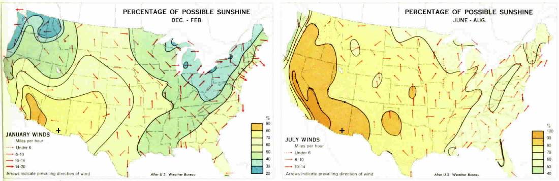
Figure 1.  Possible sunshine maps for the United States in the winter and summer.

The "possible sunshine" parameter for the United States shows a maximum region that extends NNW from Yuma, AZ.  According to these maps Sierra Vista, AZ (cross in each panel) should have 77% and 87% sunshine for the winter and summer months.  It is my impression that prior to the monsoon season there are more clear nights than clear daytimes, but during the monsoon season the reverse is true.

Here's a bar graph showing the percentage of CLR nights for the past 10 months of my observations.

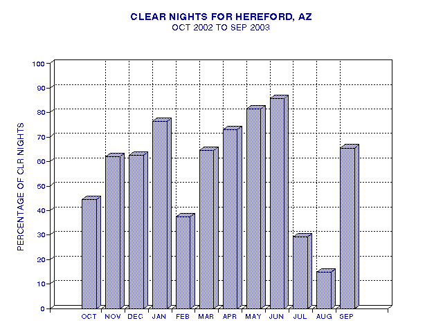
Figure 2.  Clear sky statistics for a 12-month period in Hereford, AZ (near Sierra Vistta,AZ) .

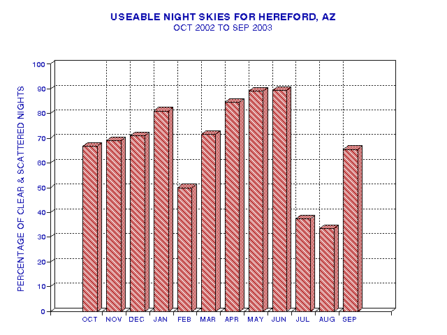
Figure 3.  Percentage of nights that were "useable" (CLR  or SCT) in Herefored, AZ during the past 12 months.

As expected, February and July/August have the fewest clear nights, and they also have the fewest "useable" nights (CLR or SCT).  The February minimum is caused by the "Pineapple Express" westerlies that bring Pacific storms through Southern California and into Southern Arizona.  The July/August minimum is due to the "monsoon season" that is caused by a summer high over the Central U.S. that pulls moist Gulf of Mexico air northwestward into Southern Arizona.  According to this graph the best months for astronomy in Sierra Vista area are May and June, right before the summer monsoon.  The worst months, again, are February and July/August.

How do the sunshine maps compare with the CLR, SCT and BKN statistics for Sierra Vista during the recent observing period?  Any comparison will require that we compare "possible sunshine" with "possible starshine."  CLR nights correspond to 100% of possible starshine,  SCT corresponds to ~70% starshine (i.e., 100% minus halfway between 10% and 50%), and BKN corresponds to ~30% starshine.  The following graph is a plot of "possible starshine" percentages for the 10-month observing period of this analysis.

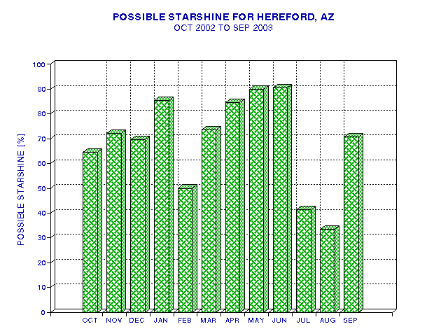
Figure 3.  Possible "starshine" at Hereford, AZ during the past year.

Figure 1 predicts a Dec/Jan/Feb sunshine value of 77%, which compares with my starshine value of 68%.  Maybe this past winter in Southern Arizona was cloudier than normal.  The sunshine maps predict a Jun/Jul/Aug sunshine value of 87%.  During this past Jun/Jul/Aug there was a 55% starshine, so the observed starshine values were lower than the climate archive sunshine values.

The summer difference may be explained by the fact that there's a daily pattern for the summer monsoons, in which the mornings are sunny and cumulus developes into thunderstorms by mid-afternoon, producing horrendous rains by late afternoon.  Even though the skies remain OVC until after the 10 to 11 p.m. time of the eveing, there was sunshine in the morning.  This artifact of my comparison may account for the different values for sunshine and starshine in the summer.

It is also possible that the differences between historical values for sunshine and one year's values for starshine are within the normal range of yearly variation, and the past year have simply been somewhat cloudier than normal.

It is not possible to blame the poorer Clear Sky Clock performance in Southern Arizona, compared with Santa Barbara, on unusual weather patterns in Arizona during the past year.
 

This site opened:  August 1, 2003.  Last Update:  October 9, 2003