Bruce L. Gary
Hereford, AZ
Last Updated 2004.04.20
Links Internal to this Web Page
Star field (orientation)
Blue Filter Observations
(March 15)
Establishing Unfiltered Sequence
March 20
Unfiltered Observations of Variability
April 9 Unfiltered
Observations of Variability
Results of My April
17/18 (AAVSO-Coordinated) Observations
Results of My April
19/20 (AAVSO-Coordinated) Observations
Other BZ UMa Links (External)
Introduction
The "dwarf nova" BZ UMa underwent a 5-magnitude outburst in late February, 2004 and within a few days it had faded ~4 magnitudes (to 15.5). A much slower fading followed, and it is now at ~16.5 magnitude. Although it is currently quiescent, there is strong evidence that it is "flickering." Many people are actively investigating this star's brightness behavior and this web page describes my efforts to document the magnitude and possible preiodicity of the quiescent flickering. More background information for BZ UMa is given at the end of this web page, as is a description of my hardware.
Star Field
and AAVSO Suggested Reference Stars
BZ UMa is located in Ursa Major, and has coordinates RA = 08:53:45,
Dec = +57:48:36 (epoch 2000). The following image shows a quiescent BZ
UMa in relation to nearby stars.
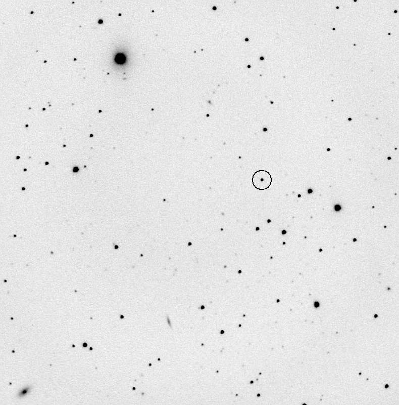
Figure 1. Unfiltered image of BZ UMa (circled) and nearby stars
within a FOV = 15.0 x 15.2 'arc. The "limiting magnitude" is 21.9 (SNR=3,
the faintest stars have a magnitude of ~21.5). North is up, east to the
left. Atmospheric seeing was average (FWHM = 3.8"arc). [Celestron
14-inch, CGE-1400, Cassegrain configuration: focal reducer, SBIG AO-7 tip/tilt
image stabilizer, SBIG CFW-8 and ST-8XE CCD, unfiltered; 69-minute total
exposure (average of 23 median combined triplets), Hereord, AZ]
Anre Henden has produced a BV photometric sequence for the BZ UMa region,
and the AAVSO finder chart with this sequence information is reproduced
below.
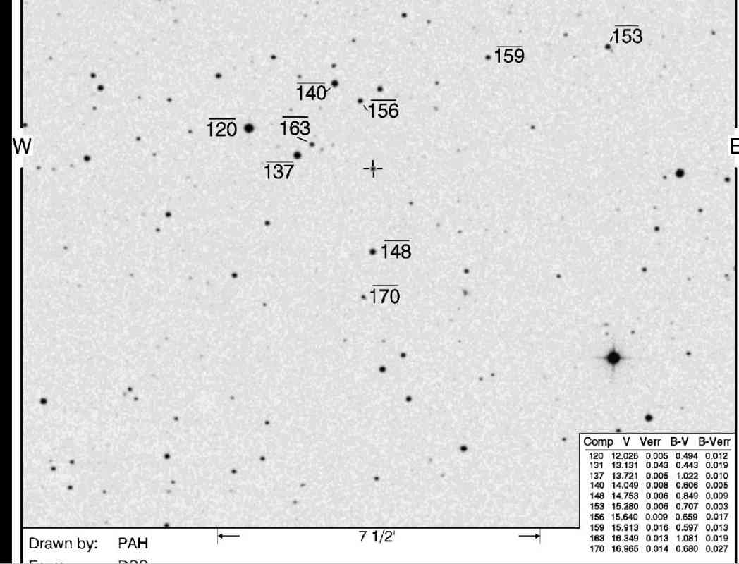
Figure 2. AAVSO finder chart (cropped image) showing most of the suggested "comparison stars" with their V and B-V magnitudes based on Arne Henden observations. North is down, east is to the right (i.e., a 180 rotation with respect to the previous figure).
My observations confirm the relative magnitudes of most of the AAVSO "comp
stars" and by inference confirms Arne's multi-night assessment that they
are non-variables. This is shown for the B-magnitudes in the next figure.
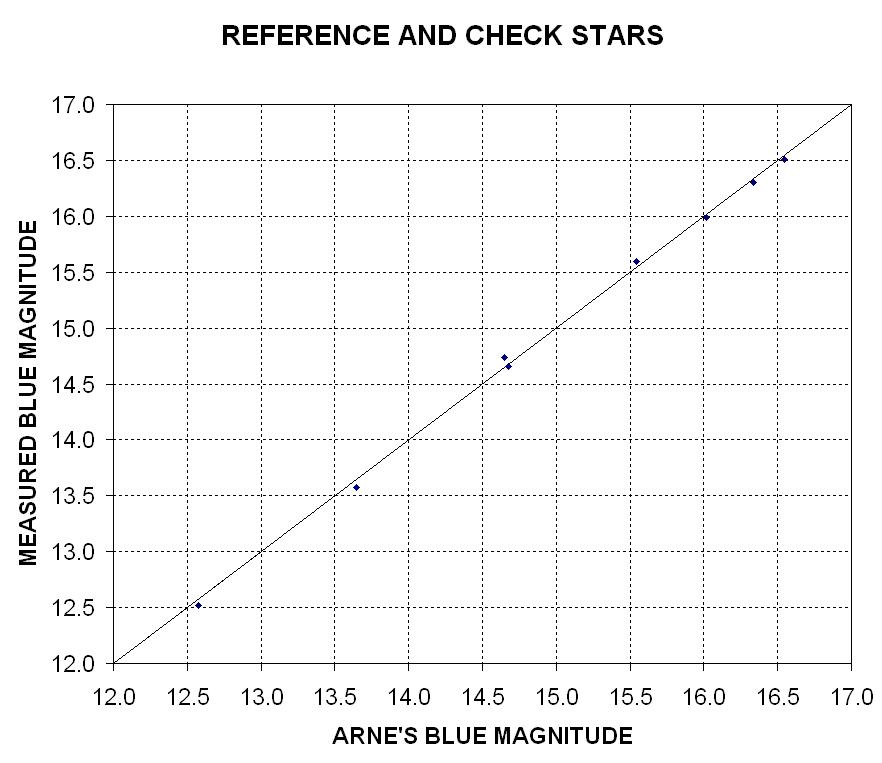
Figure 3. My measured versus Arne's measured B-filter magnitudes for 8 of the AAVSO suggested "comp stars." My magnitude scale was set by forcing 4 of this set of stars to have the same average as Arne's measrurements.
My purpose in producing this graph was to confirm that the AAVSO suggested
comp stars were not variable, and seccondarily to confirm that my system
was linear.
March 15 Blue Filter Observations
My initial observing goal for BZ UMa was to confirm a previously measured
flickering with a B-filter during a 4-hour observing interval that showed
variations of ~0.1 magnitude (Kaluzny, 1986).I was able to observe with
a B-filter for only 2 hours, when it became apparent to me that my SNR was
not sufficient to detect 0.1 magnitude variations. These measurements are
shown in the next figure.
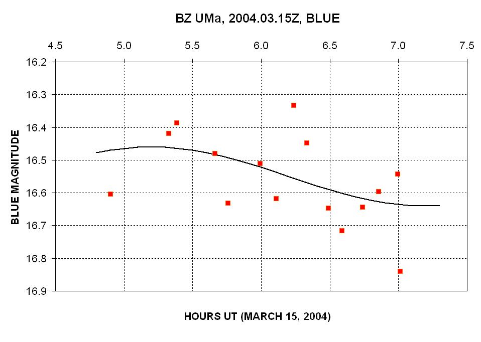
Figure 4. B-filter monitoring for a 2-hour interval during quiesence.
Although I had insufficient SNR to detect 0.1 flickering variations on
a time-scale short compared with the rotation period (1.6 hours) there
exists a variation with a weakly established range of 0.2 magnitude which
was not present in check stars of comparable magnitude (available upon
request). After completing this B-filter observation I decided to switch
to unfiltered observing of BZ UMa.
Establishing
an Unfiltered Sequence
Since my observing objective is to attempt a measurement of small brightness changes of BZ UMa, and since I showed that my telescope aperture is too small for confirming previously reported B-filter flicker, I decided to switch to unfiltered observations. For this I needed a magnitude scale, yet unfiltered magnitude scales are never created (since they would apply to only the system that created it, given the great variation in spectral response of diffeerent systems across the entire unfiltered spectrum). I created an unfiltered magnitude scale by adopting the V-magnitudes of 4 AAVSO "comp stars" and zero-shifting my observed magnitudes for these stars to achieve average agreement. The set of 4 stars had unfiltered magnitudes that differed from Arne's V-magnitudes by small amounts (RMS difference = 0.08 mag), which is to be expected when the star's spectral types are similar (which they were). The following image is annotated to show the unfiltered magnitudes I determined for 8 AAVSO comp stars (that is valid for a system with my spectral response).
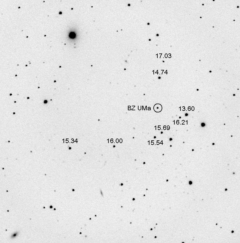
Figure 5. "Unfiltered sequence" that is internally consistent
using my telescope system. Four stars were used to establish a zero shift
to achieve average agreement with Arne's V magnitude scale (13.60, 15.69,
16.00 and 14.74). [Same starting image as Fig. 1]
To the extent that my telescope system has a spectral response similar
to the systems inuse by other observers this "unfiltered sequence" would
be prefereable for use compared with the V-magnitude sequence. It is preferable
in two respects. First, the observer can more quickly assess the linearity
of an image by plotting measured versus expected magnitudes and inspecting
for departures that form a pattern (consistent with saturation, for example).
Second, comparing observations from different observers with partial of
missing temporal overlap, the task of zero-shifting each observer data set
will involve smaller adjustments if their reproted BZ UMa magnitudes use
the "unfiltered sequence" instead of the V sequence (assuming the observed
unfiltered).
March 20 Unfiltered
Observations
On March 20, 2004 I observed BZ UMa for 2 hours using a clear filter (unfiltered)
and 1-minute exposures. Since I always perform a median combine of 3 or
more images before doing photometry, the temporal resolution is slightly
more than 3 minutes. The following figure is a screen shot of MaxIm DL's
photometry tool analysis of 22 median combine triplets, using the "unfiltered
sequence" described in the previous section.
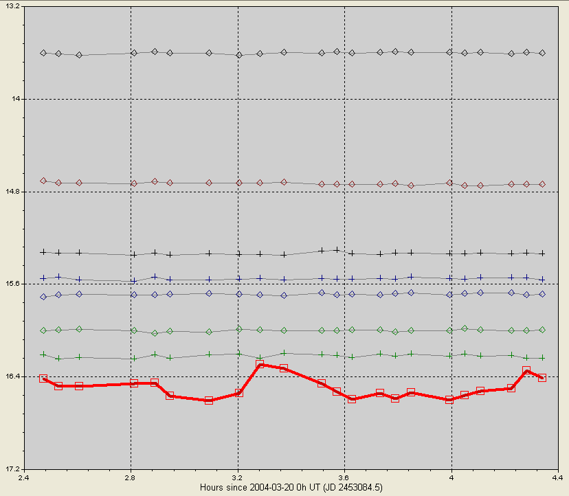
Figure 6. Unfiltered magnitude versus time for 4 refernce (comp)
stars, 3 check stars and BZ UMa (red trace) during a 2-hour interval on
March 20, 2004.
It is apparent in the above figurethat BZ UMa exhibits a greater amount
of variation than the other stars. However, it should be taken into consideration
that the fainter the star the greater the variation, due to SNR considerations.
Thus, I analyzed the RMS variation off the average for each star, and plotted
this parameter versus brightness in the next figure.
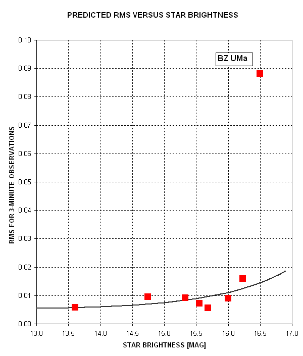
Figure 7. Unfiltered RMS (with respect to average) for the 8 stars
studied in the March 20 observations. The high value for BZ UMa is well
above a model fit to the other stars which implies that it was actually varying
during the observing interval.
In the above figure I used a model RMSfit = const1 + const2/intensity,
where "intensity" is 2.512^(15-mag) and "const1" and "const2" are two arbitrary
constants adjusted to produce a good fit the reference and check stars RMS
values (using "15" in "15-mag" is arbitrary since any value different from
15 will simply call for a different "const2" value; 15 was chosen for convenience).
Given that BZ UMa has an RMS that is statistically greater than the expected
(model fit) value, I conclude that it exhibited real variations that were
measured. Whereas the compnent of RMS variation that cannot be explained
by the model fit is only 0.087 mag (sqrt{0.088^2 - 0.015^2}), since this analysis
establishes that real variations are present it is permissible to interpret
the Fig. 6 plot of BZ UMa variations in such a way that a hypothetical smoothed
plot of BZ UMa magnitude versus time will exhibit the expected residual RMS
variation of 0.015 magnitude. Doing this "by eye" it is apparent that most
of the BZ UMa variation is real, and has a range of ~0.25 magnitude.
Note that the March 20 observing interval is longer than the rotation
period, so any rotation-related variation would be captured by this observing
run.
April 9 Unfiltered
Observations
The next two figures are analogous to the previous two, and they are based
on a 1.6-hour unfiltered observing session on April 9, 2004 UT .
Figure 8. Light curve for BZ UMa (red filled squares) and 4 reference
stars and 4 check stars. (Note that negative magnitude is plotteed since
the spreadsheet I used for this could not reverse the Y-axis values.) Each
datum is photometry for an image that is a median-combined triplet where
each image for the triplet is a 1-minute exposure, producing a plot with
3-minute temporal resolution.
Notice that BZ UMa has the same average magnitude on April 9 as on March
20, and it exhibits a range of variation that is similar to that of March
20.
Figure 9. RMS differences for each star (with respect to that star's average magnitude) versus star magnitude. The model fit was adjusted to agree with the reference and shcek stars. BZ UMa is plotted as a filled red square.
As on March 20, BZ UMa exhibits a RMS about its average that is greater
than would be expected (for its magnitude), although on this date the discrepancy
is less. This observing session has a predicted RMS variation for a star
with BZ UMa's brightness that is 0.025 magnitude (instead of the March 20
expected RMS of 0.015 magnitude). The predicted RMS at mag 16.5 is higher
than for the March 20 observations probably because of the presence of thin
cirrus that kept drifting though the region of interest. Nevertheless, the
difference between measured and expected RMS constitutes strong evidence
that BZ UMa exhibits real variations, and again, referring to Fig. 8, these
variations were ~0.25 magnitude on April 9. This is the same level of variation
as on March 20.
Upcoming AAVSO-Coordinated Intensive Observing Sessions
The AAVSO is planning a coordinated world-wide intensive observing session
to establish a good quality fluctuation light curve for two 24-hour sessions.
These are described at the following AAVSO web site:
http://www.aavso.org/news/bzuma.shtml
Lots of plans, but Murphy's Law kicked-in.
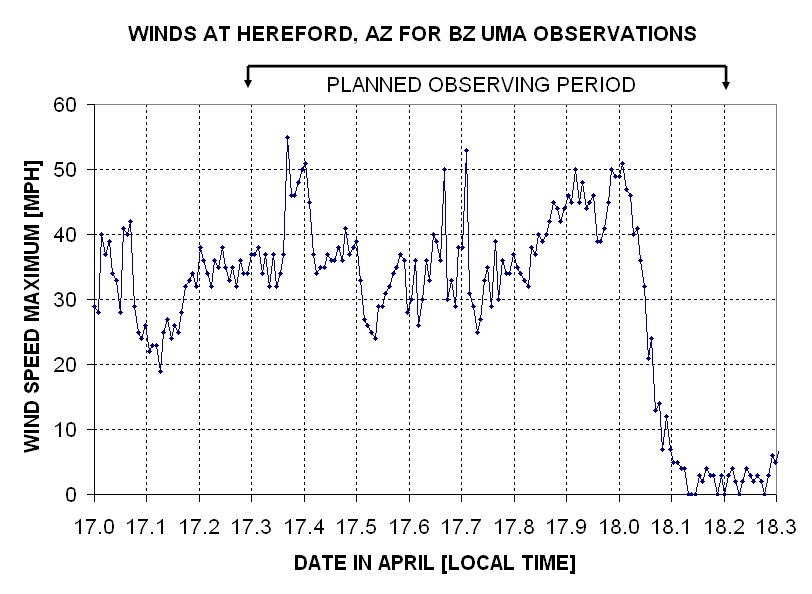
Figure 10. Winds during the scheduled observing period for April
17/18.
The following observations were made with Dave Healy's "Junk Bond Observatory"
20-inch Ritchey-Chretein telescope in Hereford, AZ. The seeing was poor (FWHM
= 4.5 to 5.2 "arc) yet the SE precision of 30-second unfiltered exposures
was good (0.04 mag). Since this telescope is inside a dome there are fewer
cosmic ray defects and it is safe to perform photometry on individual 30-second
images (without median combining 3 or more).
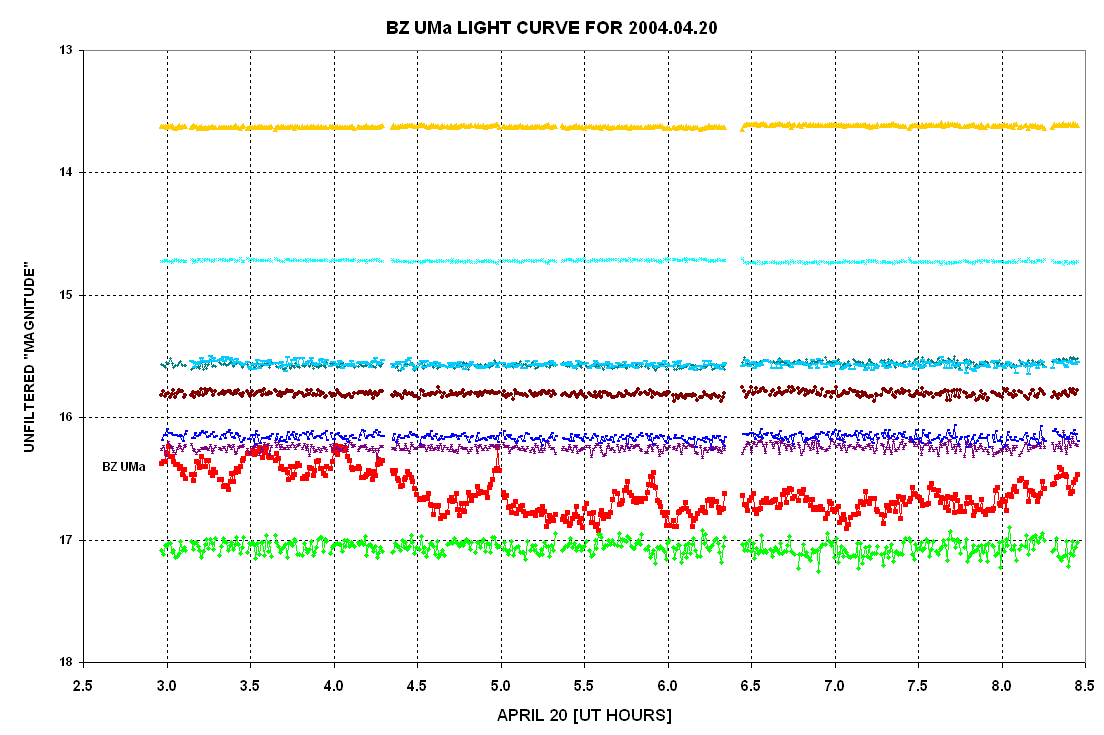
Figure 11. Brightness of BZ UMa (red symbols), two reference stars
(brightest two) and 6 check stars during the April 20 AAVSO coordinated observing
period. Each datum is from a 30-second exposure.
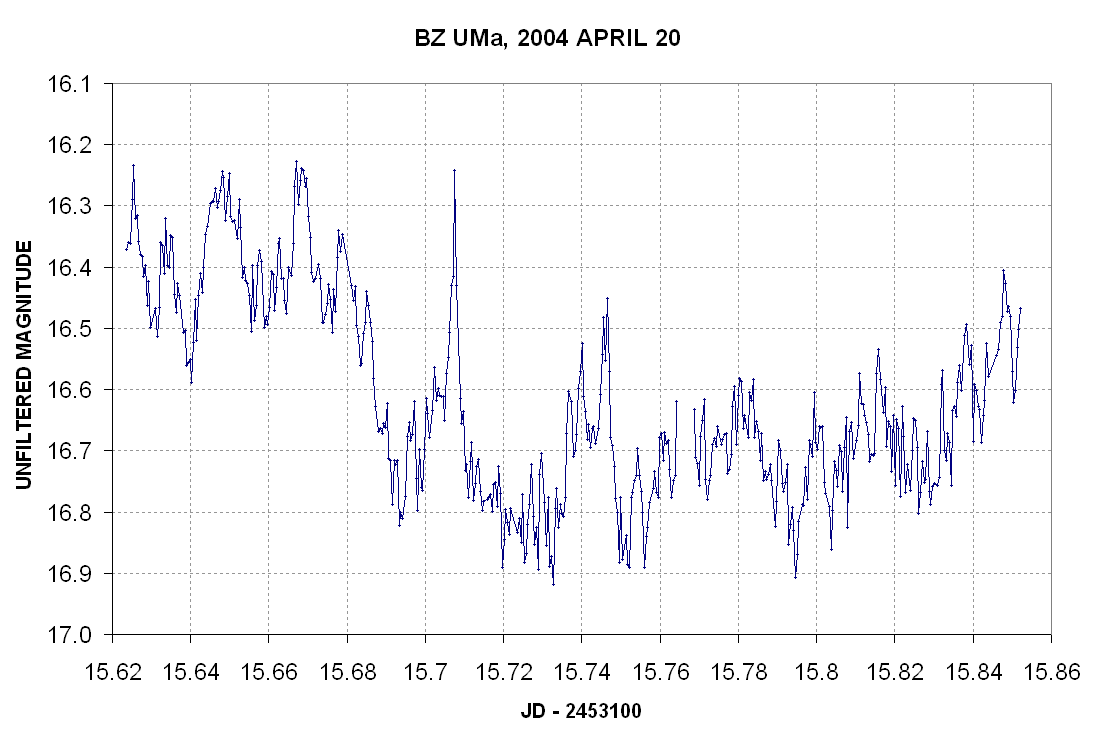
Figure 12. Brightness of BZ UMa during the April 20 AAVSO coordinated
observing period. Each datum is from a 30-second exposure
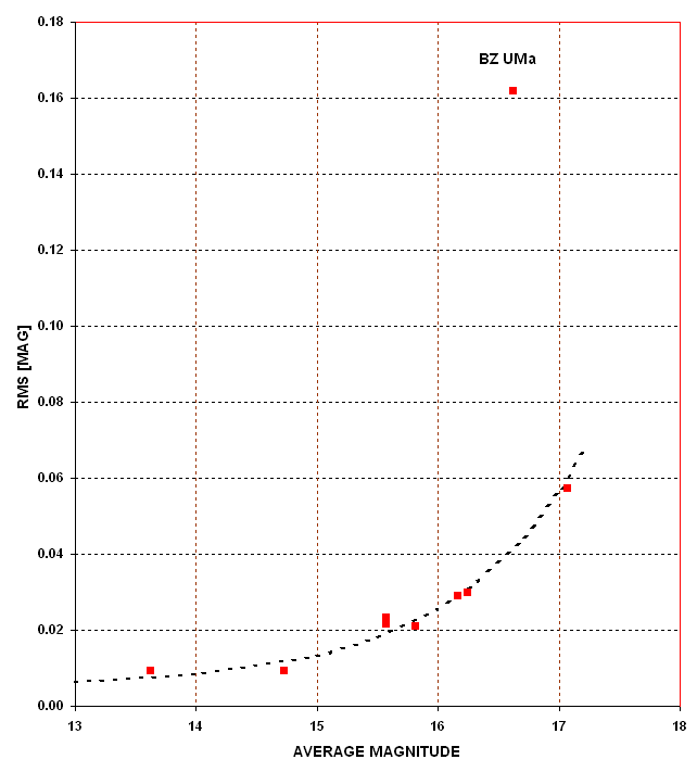
Figure 13. RMS variation of measured magnitude versus average magnitude
for the 2 reference star, 6 check stars and BZ UMa (the "outlier" having RMS
= ~0.16 mag).
The RMS performance for a star with an average magnitude of 16.5 is 0.04
mag. This compares with 0.015 mag RMS when I used my 14-inch Celestron
with three 1-minute median combined images on March 20. The 20-inch telescope
30-second exposures contain 1/3 as muny photons as the 14-inch 3-minute total
exposure images, so in theory the two RMS perforamces should differ by the
ratio 1.7 (square-root of 3), with the 20-inch 30-second images having a
higher RMS. The fact that it had 1.5-times higher than expected RMS may
be due to the poor "atmospheric seeing" for the 20-inch telescope observations.
My April 9 obsrvations were made with thin cirrus drifting through so the
0.025 mag RMS for 3-minute images for that date are probably not representative
of clear weather.
Background Information
for BZ UMa
BZ UMa is a member of a binary system with an orbital period of ~1.63 hours
according to time-resolved spectroscopy (Ringwald, et al, 1994). The
binary consists of a white dwarf and a red M5 (spectral class) dwarf that
has expanded to fill the Roche lobe. The red dwarf expansion causes occasional
transfer of gas to the white dwarf, which creates an accretion disk around
the white dwarf. This binary system is believed to belong to a class of variable
star referred to as a UG System, sub-class SU, or UGSU (according to the
literature search by Aaron, 2004). A description of these terms is given
below.
"UG System" Variable Star Description
U Geminorum-type variables, quite often called dwarf novae. They are close
binary systems consisting of a dwarf or subgiant K-M star that fills the
volume of its inner Roche lobe and a white dwarf surrounded by an accretion
disk. Orbital periods are in the range 0.05-0.5 days. Usually only small,
in some cases rapid, light fluctuations are observed, but from time to
time the brightness of a system increases rapidly by several magnitudes
and, after an interval of from several days to a month or more, returns to
the original state. Intervals between two consecutive outbursts for a given
star may vary greatly, but every star is characterized by a certain mean
value of these intervals, i.e., a mean cycle that corresponds to the mean
light amplitude. The longer the cycle, the greater the amplitude. These systems
are frequently sources of X-ray emission. The spectrum of a system at minimum
is continuous, with broad H and He emission lines. At maximum these lines
almost disappear or become shallow absorption lines. Some of these systems
are eclipsing, possibly indicating that the primary minimum is caused by
the eclipse of a hot spot that originates in the accretion disk from the
infall of a gaseous stream from the K-M star. According to the characteristics
of the light changes, U Gem variables may be subdivided into three types:
SS Cyg, SU UMa, and Z Cam.
UGSU Subclassification of UG Systems
SU Ursae Majoris-type variables. These are characterized by the presence of two types of outbursts called "normal" and "supermaxima". Normal, short outbursts are similar to those of UGSS stars, while supermaxima are brighter by 2 mag, are more than five times longer (wider), and occur several times less frequently. During supermaxima the light curves show superposed periodic oscillations (superhumps), their periods being close to the orbital ones and amplitudes being about 0.2-0.3 mag in V. Orbital periods are shorter than 0.1 days; companions are of dM spectral type;
[The two descriptions above were copied from the web page: http://www.sai.msu.su/groups/cluster/gcvs/gcvs/iii/vartype.txt which is the General Catalog of Variable Star Types web page]
Hardware, Observing Sequence and Analysis
Description
Hardware
My telescope is a 14-inch Celestron CGE-1400 (German equatorial mount)
Schmidt-Cassegrain. For these observations I am configured for Cassegrain
observing (not prime focus). I use a Celestron focal reducer, a SBIG AO-7
tip/tilt image stabilizer, a SBIG CFW-8 with Custom Scientific photometric
filters, and a SBIG ST-8XE CCD. I control the telescope, AO-7, CFW and
CCD using MaxIm DL/CCD Ver. 3.0 software. The telescope is in a sliding-roof-observatory,
SRO, located ~70 feet from my residence office, and all controls are performed
from the residence office computer through 100-foot cables, that run through
buried conduit.
Observing Sequence
I use dusk sky flats taken shortly after sunset with exposures of ~1 second
or longer. Sometimes a T-shirt aperture cover is used to avoid stars from
appearing on the sky flat images. A typical observing sequence consists
of 16 exposures: 15 "lights" and one "dark." During analysis many darks
are median combined (to elmininate cosmic ray defects). All observations
of a given object are performed at the same CCD cooler setting (to allow
combining of many dark images). I refer to the set of 16 images as
an "observing sequence." MaxIm DL/CCD automatically names observing sequences
with sequential sequence numbers.
Image Analysis and Photometry
The set of 15 light images are calibrated for flat and dark, then inspected for quality. A specific star is chosen for quality monitoring; that star's FWHM and Intensity are used to assure that no images are accepted that have poor tracking or large extinction due to drifitng cirrus clouds. Poor tracking can occur if image motion due to atmospheric waves is excessive (caused by mountain ridge 5 miles upwind of me). FWHM can occasionally worsen suddenly due to turbulence (caused by atmospheric Kelvin-Helmholtz wave breaking).
Each set of 15 images is converted to 5 median-combine triplets. In other words, calibrated images #1, 2 and 3 are median combined to produce image A; then images 4, 5 and 6 are median combined to produce iamge B, etc. These median combined triplet iamges are then analyzed with MaxIm DL's Photometry Tool (which has partial pixel and reference annulus median combine features). After selecting an "object" (BZ UMa), 4 "reference stars" (i.e., "comp stars) and 4 check stars, and enter the View window and I choose at least two aperture sets. An aperture set is a coice of aperture circle radius, gap width and reference annulus width. These three numbers, which I refer to as RGA (for radius, gap width and annulus width) produce a photometry result that is recoded as a text file (with extension CSV, standing for comma delimited values). These text files contain JD, object magnitude, reference star magnitudes and check star magnitudes. The CSV files are imported to a spreadhseet (I prefer Quattro Pro for DOS over Excell - I hate Excel, which is designed for pie-chart loving salesmen, not scientists). When first opening the spreadhseet program I first import a "seed" spreadsheet that has cell assignments that I've created for this specific task of processing CSV-files. The spreadsheet calcualtes average magnitude for each star (averaging the 2 or more RGA choices associated with each CSV-file, that I import). The seed spreadsheet has ready-made graphs for checking "measured versus expected magnitude" which are useful in identifying cases when I entered the wrong reference star magnitude in MaxIm DL's Photometry Tool. If this and other spreadsheet wuality checks are OK, I perform a "block save to file" recording of the average magnitudes for the object (BZ UMa), all reference stars and all check stars. This block save file is meant for later import to a final day's analysis spreadsheet, where the photometry results for all 16-image sequences is combined to produce a plot of an entire observing session's light curves.
Yes, this is a lot of work, but a 4-hour night's observing session can
be reduced the following day (I'm retired, so there'sno problem doing this).
http://www.aavso.org/news/bzuma.shtml
____________________________________________________________________
This site opened: April 10, 2004 . Last Update: April 20,
2004