This chapter relates world population data with
science
and technology innovations and arrives at a "per capita rate of
innovation"
graph. The "per capita rate of innovation" shows two peaks, one
starting
during the Golden era of Greece and the other starting during the
Renaissance
and peaking at the end of the 19th Century. A range of dates for the
demise
of humanity is calculated on the very speculative principle that
there's
a 50% chance that we now find ourselves between the 25th and 75th
percentiles
of the sequence of the birth dates of all humans who shall ever be
born.
In 1990 I wrote a brief version of this essay, dealing specifically
with
the statistical argument for inferring that the demise of humanity was
imminent;
it appeared in an unpublished book, Essays From Another Paradigm.
The present chapter is adapted from a 1993 expanded essay on the
same
subject.
Population Versus Time
Table 1 is a compilation from many sources of
the
world's population for 26 epochs. The original literature almost
never
provides uncertainties, but if scatter is any guide the uncertainties
range
from 3% during this century, to ±3 dB (+100/ 50%) at 8000 BC,
and
±5 dB at 100,000 BC.
Table 1
Year Pop’n Year Pop’n Year Pop’n
[AD] [millions] [AD] [millions][AD] [millions]
100,000 0.5 1500 440 1950 2530
50,000 1 1600 470 1960 3000
18,000 3 1650 545 1970 3600
8,000 9 1700 600 1980 4400
7500 10 1750 725 1990 5300
3000 30 1800 907 2000 (6380)
1000 110 1830 1000 2010 (7300)
0 200 1900 1600 2025 (8500)
1000 340 1930 2000 2038 (8500)
A 10th order polynomial fit to the relationship
of
"log of population" versus "log of time" is given at the end of this
chapter.
It has been used to perform integrations from the distant past to dates
of
interest. The following figure plots the tabulated data (symbols) and
the
10th order fit (trace).
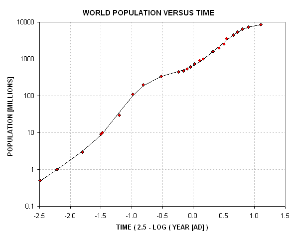
Figure 15.01. World population versus time, using a special Log scale for time. The trace is a 10th order polynomial fit, used to assist in later calculations.
Figure 15.02. Adopted world population, with arbitrary choice of year for x axis representation.
Birth and Survival Rates
Before proceeding to the calculation of the
integrated
number of human live births and adults, it is necessary to address the
issue
of birth and survival rates. The simplest method for calculating the
integral
of population from some arbitrary start time to x axis time is to
multiply
"crude birth rate" times "population" times "time interval." I've
adopted
a crude birth rate table that starts at 45 births per thousand at
100,000
BC, and decreases monotonically to 26 births per thousand in 1993. It
has
been established that the main decrease started at approximately the
time
of World War II, when it had a value of 38 births per thousand. Not all
babies
live to adulthood. Throughout the world prior to the 18th Century
approximately
25% of babies survived to adulthood (taken to be the age when
reproduction
begins, about age 18 in primitive societies, and age 13 in developed
world
societies). In other words, in the natural order of things
approximately
3/4 of all newborns are destined to die before adulthood! Since the
18th
Century the developed world has achieved a much better survival rate,
approximately
95% (versus 25%). But still, the undeveloped world (about 71% of the
world's
population) has survival rates of approximately 30 to 35%. The adopted
world
average survival rate conforms to estimates of the fraction of the
world's
population that is "undeveloped" versus "developed." The adopted birth
and
survival rates are shown in the following figure.
Figure 15.03. Adopted crude birth rate (solid) and survival rate (dashed).
Integrated Population Versus Time
The previous graphs illustrate time interval
averages
for population, birth rate and survival rate. These are combined to
calculate
the integrated number of births from 100,000 BC to x axis time. In the
following
figure the upper trace is labeled "live births." Thus, this trace is
the
total number of live births from 100,000 BC to x axis time. Note
that
the x axis is neither linear nor logarithmic, but corresponds to dates
in
the original population data, above.
Figure 15.04. Integrated number of live births (dotted) and integrated number of humans reaching adulthood (solid).
Note the solid trace, the integral of adults
who
have inhabited the earth from 100,000 BC to x axis time. To calculate
this
it was necessary to use the estimated survival rate versus time (the
lower
trace in Fig. 15.03). The number of "adults" that have inhabited the
world
is about 33% of the number of all humans born. For the epoch of these
calculations,
1993, the total number of "live births" was 60.3 billion, and the total
number
of adults who have ever lived (to 1993) is 19.6 billion.
As an aside, Fig. 15.05 is a plot of the D/L Ratio, defined as the ratio of dead to living. This parameter was apparently treated by Asimov (reference unavailable).
At the time of this writing (2001) the D/L Ratio is about 8.6. Figure 15.06 shows how the ratio "people aliveat date" to "total births to date" ratio has varied over time.
Figure 15.05. Ratio of dead to living (solid trace) versus time.
Figure 15.06. Percentage of "all births" represented by "people alive."
In the year 2006, when 6.8 billion people are
supposedly
alive; they constitute 11% of all people who have ever been born.
The following figure is an alternate presentation of the data in Fig. 15.04, with a rescaling of the y axis so that in 1993 the integrated number of people is 100%.
The following figure is an alternate presentation of the data in Fig. 15.04, with a rescaling of the y axis so that in 1993 the integrated number of people is 100%.
Figure 15.07. Integrated number of human live births and humans reaching adulthood, normalized so that 1993 has 100% of the integrated numbers.
The above figure plots the "integrated number
of
people" as a percentage of the 1993 numbers. The "live births" and
"adults"
traces cross at 1993, by definition. These traces can be used to define
what
I shall call the "Humanity Time Scale." Which of these traces should be
used?
The "live births" trace has fewer assumptions; just the population
versus
time and the birth rate versus time, both of which are well
established.
The "adults" trace may be more appropriate for what we are going to do
with
the Humanity Time Scale as it reflects the number of humans who have
lived
long enough to think about the world, and contribute to it's
irreversible
legacy of innovations. The weak part of the argument for adopting the
"adults"
trace is that it depends on survival rate, which is an assumed
parameter.
It is less well established than the other two properties. The halfway
points
(the 50% level) for the two traces are at 834 AD and 1118 AD, for "live
births"
and "adults."
The following figure is a plot of "% of adults before date" versus year for a set of arbitrarily chosen integer dates.
Figure 15.08. Integrated number of human adults born before (arbitrarily selected) x axis years.
It is slightly easier to use this graph to determine dates before which specified percentages of all human adults were born. For example, 80% of adults lived prior to the year 1891 AD, and 82% of adults lived before 1908 AD. Thus, 1891 to 1908 AD is a "2% of adults" interval (corresponding to 80 to 82% of adults). There are 50 such 2% intervals prior to 1993, and each has corresponding beginning and ending dates.
Innovation Data
“Asimov's Chronology of Science and Discovery" (198?, 1994) has been analyzed to determine how many innovations belong to each of the 2% intervals. Asimov's list has 1478 entries, from 4 million BC to 1991. For the time span 100,000 BC to the present, there are 1474 items. A histogram was created showing the number of items for each 2% date interval. For example, for the 2% date interval 1891 to 1908 AD, there were 120 citations in Asimov's list. As there are 2% of 19.6 billion adults during each 2% interval, or 392 million adults, the number of innovations per billion people can be calculated by dividing the number of citations by 0.392. The results of this conversion are presented in the following figure.
Figure 15.09. Number of innovations per billion adults for each 2% interval of the Humanity Timescale.
The first peak, at 28%, the 2% interval of 26% to 28%, corresponds to 500 BC to 290 BC. The minimum at 38% corresponds to the dates 390 AD to 500 AD. The abrupt rise after 60% corresponds to the mid 15th Century, which is when the Renaissance began (1453 AD). The peak at 82% (corresponding to the 80 to 82% time interval cited above) is for the period 1891 to 1908 AD. The steady decline since 1908 has progressed to a level corresponding to that of the 16th Century.
Weighted Average Innovation Rate
About 96% of Asimov's science and discovery citations belong to a category that requires formal education, by my cursory review. It is thus natural to ask how many "literate" people there have been over time, and how does the innovation rate look when it is normalized to the relative numbers of literate people? Better, how does the innovation rate look when it is normalized using a 96% weight for the literate population and a 4% weight for the illiterate population?
To normalize the innovation rate traces to the population of literate adults it is necessary to adopt literacy rates over time. I have chosen to do this on a region by region basis, since literacy commences at different times in different world regions. It is also necessary to estimate regional population traces. I have chosen 9 world regions for this task. Figure 15.10 shows the population of 5 regions (the most populace), and Fig. 15.11 shows the population of the remaining 4 regions.
Figure 15.10. Population breakdown for 5 regions and their total.
Figure 15.11. Population breakdown for another 5 world regions, and their total.
Notice that in Fig. 15.10 Europe experienced two population peaks before the Renaissance: in 200 AD and 1300 AD. There are population collapses after each peak. The first collapse must have something to do with the inability of urban centers to support large populations (the population of Rome fell dramatically, for instance), while the second collapse was produced by the scourges of the Black Death. In Fig. 15.11 there is one (documented) population collapse, starting in 1500 AD, caused by diseases brought to the New World by European explorers and settlers. The population rise starting in 1750 is due to massive migrations of Europeans.
It was not possible to find literacy rates for all these regions for the times of interest. After the suggestion of Dr. Kevin Pang, I adopted the procedure of estimating literacy rate by assuming that most urban populations are mostly literate while most of the rural populations are illiterate, at least until recent times. Urban and rural statistics are easier to estimate, so this procedure can be used for more regions and can be extended back in time to the adoption of writing in each region. In constructing these tables it was assumed that approximately 50% of the pre 15th Century urban population was literate, and approximately 1% of the rural population was literate. After 1500 AD a gradual increase in the two literacy rates are adopted, ending with a present day 90% and 40% (weighted average of all regions).
Other minor adjustments were made as an attempt to represent "realism." For example, for the Americas the literacy rate was allowed to climb from zero during the first Century AD, when the Mayan “civilization” is thought to have adopted writing. The Americas literacy rate remained at low levels during the pre Columbian era, and rose rapidly during the European immigration. Similar "origins" of literacy are attributed to China in the 17th Century BC, and "Europe" (actually Mesopotamia") during the 4th Millennium BC. Regional literacy rates were combined with regional populations to produce a global literacy rate and total number of literate adults, which is shown in Fig. 15.12.
Figure 15.13 is innovation rate per literate adult. It is a renormalization of Fig. 15.09, using the global literacy rate as a normalizing factor; so it thereby retains the property of showing how many innovations were produced per million literate adults who lived during the “equal increment of adults” intervals.
It is remarkable that after the classical Greek period the rate of innovations is level at about 50 per million literate adults until well into the 19th Century. This could be the source of interesting speculation, but for now I will defer. The pre Greek times produced innovation rates comparable to those of the Greek era, but this feature is less robust for several reasons: 1) there are fewer innovations in the numerator, and 2) there is great uncertainty in estimating (or even defining) literacy during this time.
Figure 15.12. Estimated global literacy rate and total number of literate adults versus time.
Figure 15.13. Innovation rate per literate adult.
The drop in innovation rate since 1800 is attributable to two equally important factors: 1) a population that rose by a factor of 5.5, and 2) literacy rate grew by a factor of 3.8. Since both factors move the innovation rate trace in the same direction, a factor of 21 decrease is predicted due to these two considerations alone (while a drop of 15 to one is observed).
Figure 15.14. Innovation rate per billion population, weighted average of rates for literate and all adults.
This figure is a plot of the innovation rate using the weighted average of 4% for illiterates and 96% for literates. This trace is based on the concept that the literate person is 24 times as likely (96/4 = 24) to produce an innovation (that Asimov would include in his list) compared to the illiterate person. This presentation is the "fairest" way that I can think of for representing innovation rate using Asimov's compilation as the measure for significant innovations.
The Two Major Peaks in Innovation Rate
There are still two peaks in Fig. 15.14, as there were in Fig. 15.09. The classical Greek peak in relation to the 19th Century peak is 13% in Fig. 15.09, and 17% in Fig. 15.14. Normalizing by a weighted average of literate people and illiterate people's overall productivity did not significantly change the relative appearance of the two versions. The Greek peak endures for about 4 centuries, from 500 BC to 90 BC. The 19th Century peak occurs between 1550 AD and 1993 AD, approximately, which is about 4.5 centuries long. Thus, the durations are approximately the same in terms of normal, calendar time, being 4 or 5 centuries. I will refer to this most recent peak as the Renaissance/Enlightenment innovation peak.
There is another similarity between the Greek and Renaissance/Enlightenment peaks. They are both accompanied by an increasing population, and the Greek population rise reaches a maximum some centuries later. The Greek infusion of new ideas was exploited by the Romans, who made it possible for populations to increase until a collapse after 200 AD. The population maximum occurred 5 centuries after the innovation peak. Figure 15.15 illustrates this.
Figure 15.15. European population in relation to global weighted average innovation rate, showing that the "Greek" innovation peak is followed 5 centuries later by a "Roman" population peak.
Figure 15.16. A 1400 year expanded portion of the previous figure, centered on the Greek innovation peak.
Figure 15.16 shows a 1400 year expanded portion of the previous figure, centered on the Greek innovation peak. The Roman population peak follows the Greek innovation peak by 4 to 6 centuries.
Figure 15.17 shows another 1400 year period, centered on the Renaissance/ Enlightenment innovation peak. Clearly, this dynamic cycle is still unfolding and we alive today are naturally interested in its outcome.
Figure 15.17. Another 1400 year period, but this time centered on the Renaissance innovation peak.
It is inevitable that the still-unfolding Renaissance/Enlightenment innovation peak will be followed by a population peak, and I conjecture that its timing will be similar to the timing of the Greek innovation and Roman population peaks. We do not know the future, but some population projections resemble the plot in the next figure, with a population peak in ~2200 AD, and a collapse afterwards.
Figure 15.18. The same Renaissance 1400 year peak period, but with a future population trace, showing a population peak aafter the innovation peak.
Actually, this particular future population curve is a special one, for which I shall present an argument in the next section. Note, for now, that the population peak occurs only 3 centuries after the innovation peak, whereas the Roman population peak followed the Greek innovation peak about 5 centuries. By analogy, the currently unfolding population explosion in the undeveloped world owes its existence to the Renaissance/Enlightenment innovation peak at the end of the 19th Century.
It is also interesting that for both pairs of innovation/population peaks, the innovations and population growth occurred in different parts of the world. The spread of technology from the site of its origin allows other populations to grow almost as surely as it allows the innovating population to grow. This is reminiscent of the old saying: "When the table is set, uninvited guests appear."
Random Location Principle and Forecasting the Future Population Crash Date
It is perhaps important to put the upcoming population crash scenario to the test of what I shall refer to as the Random Location Principle. After I performed the analysis presented here I learned that the subject had been discussed in a late 1980's publication and was referred to as the “Anthropic Principle” (erroneously, I think). The Random Location Principle states that "things chosen at random are located at random locations." This innocent sounding statement is not trivial. It can have the most unexpected and profound conclusions, as I will endeavor to illustrate.
Before applying the Random Location Principle (RLP) to the population crash question, let us consider a simpler example that illustrates the RLP concept. Consider the entire sequence of Edsel cars built. Each car has an identification number, thus allowing for the placement of each Edsel in a sequence of all Edsel cars. Assume for the moment that we don't know how many Edsels were manufactured, and let's try to think of a way to estimate how many were manufactured by some simple observational means. Suppose we went to the junk yard and asked to see an Edsel. Assuming we found one, we could read the identification number and (somehow) deduce that it was Edsel #4000 (the 4000th Edsel manufactured). Would this information tell us anything about the total number manufactured? Yes, sampling theory says that if we have one sample from the entire sequence, and if it is chosen at random, then if we double the number in the sequence we'll arrive at an estimate of the total number in the sequence. In other words, doubling 4000 gives 8000, which is a crude estimate of the length of the entire sequence.
Sampling theory goes further, and states that we can estimate the accuracy of our estimate. Namely, we can assume that a sample chosen at random has a 50% probability of being within the 25th and 75th percentile of the entire sequence. If 4000 were near the 25th percentile, then the sequence length would be 4 times 4000, or 12,000. If 4000 were near the 75th percentile, the sequence length would be 4000 * 1.333, or 5300. So, with just one random sample, the number 4000 in the sequence, we could infer that there's a 50% probability that the entire sequence length is between 5300 and 12,000. Moreover, there's a 25% probability that the entire sequence length is either less than 5300, and a 25% probability that it is greater than 12,000.
Now we’re ready to apply this principle to the human sequence. Assume every human birth is assigned a sequence number. Let's delete people who fail to reach adulthood, so our new sequence is for all people born who eventually become adults. The next step is going to be difficult for most readers, but I want to try it. Imagine that the future exists in some sense. It's like watching a billiards game and having someone exclaim that while the balls are moving the future motion of the balls is determined. Thus, after the balls are set in motion the unfolding of future movements and impacts is determined. For physicists it is somewhat straightforward to conceive of the universe as a giant billiards game, set in motion by the Big Bang 13.7 billion years ago. So imagine, if you can, that there is a real sequence of unborn people who will be added to those already born, and that this sequence is somehow inherent in the present conditions. If it helps, think of time as a fourth dimension, and the entirety of the future is just as real as the entirety of the past, and the NOW of our experience is just a 3 dimensional plane moving smoothly through the time dimension. If you can accept this concept, then the rest is easy.
Each person is just one in a long sequence of people comprising the entirety of Humanity. Few people can expect to find themselves at a privileged location in this sequence; rather, a person is justified in assuming that they are located at a "typical" location in the sequence. For example, there's a 50% chance that you and I are located between the 25th and 75th percentile along this sequence of all humans. If we are near the 25th percentile, and since 19.6 billion adults were born before us, we could say that another 58.8 billion adults remain to be born (i.e., 3 x 19.6 = 58.8). Or, if we happen to be near the 75th percentile, we could say that another 6.5 billion people remain to be born (i.e., 19.6 / 3 = 6.5). In other words, there's a 50% chance that the number of humans remaining to be born is between 6.5 billion and 58.8 billion. To convert this to calendar dates, we need to experiment with future population curves to find those which end with the required hypothesized number of future adult births.
Consider the future population trace in Fig. 15.18 that goes to zero in 2400 AD. Integrating it to 2400 AD yields 35 billion new adults. If this is humanity's destiny, then those born in 1993 would be at the 56% location in the entire Humanity sequence. Or, those who were born in 1939, as I am, would be located at the 49% location of the entire Humanity Birth Sequence. These locations are definitely compatible with the Random Location Principle, and the population projection that goes to zero in 2400 AD is an optimal candidate to consider, since it places today's adults near the mid point location of the Humanity Birth Sequence.
However, we are searching for a population curve that has an integral of 6.5 billion new adults, and also a curve with an integral of 58.8 billion. Through trial and error I have found two curves that meet these requirements, and they are presented as Fig. 15.19.
The curve with a population collapse to zero in 2140 corresponds to the hypothesis that we are currently near the 75% location in the Humanity Birth Sequence. The population collapsing to zero at 2400 AD is a most likely scenario, and corresponds to our being near the 50% location. And the right most curve, with a population collapse to zero at 2600 AD, corresponds to our current location being near the 25% location. There is a 50% chance that the collapse will occur between the two extremes. Thus, by appealing to the Random Location Principle, we have deduced a range of dates for the end of humanity!
Figure 15.19. Three future population scenarios, encompassing 50% of what is forecast by my usage of the Random Location Principle. See text for disclaimers.
The future population shapes can be rearranged, provided areas are kept equal. Thus, the real population curve is likely to have a small "tail." I would argue that after such a colossal collapse the people surviving and living in the tail would be genetically and culturally distinct from today's human. Following the example of Olaf Stapledon, in Last and First Men (1931), humanity after the collapse will enter a transition from a First Men phase to a Second Men phase. New paradigms will define the new man.
Final Humanity Time Scale
The following table lists equivalences of "YearAD" and "Humanity Time Scale %." The table extends to 200%, corresponding to the "most likely" population crash date of 2400 AD.
The following figure is a visual representation of the Humanity Time Scale described by the equations (modified so that the year 2000 AD corresponds to the 100% point on the scale), presented in this chapter's appendix, below.
HUMANITY TIMESCALE
Figure 15.20. Humanity Time Scale. Left scale is for past, right is for past and future, and assumes humanity (as we know it) ceases after 2400 AD. Equal intervals along the vertical scale correspond to equal numbers of adults in the entire sequence of births leading to adults
Caveat and Comment Concerning Humanity's Collapse
The population collapse suggested by the "Random Location Principle" is clearly speculative! Its claim for consideration hinges on the applicability of the Random Location Principle to the situation of a sentient being posing the question "where am I in the immense stretch of humanity?" I suppose the conventional wisdom, if someone representing it were pressed to respond to such a question, would say that we are now close to the very beginning of this immense sequence, and that humanity may exist forever. In addition, that person would say, when our sun explodes in 5 or 6 billion years, humans will have migrated to other star systems, and will have secured its rightful place as an immortal cosmic species.
Well, that optimistic belief requires a response to the following: "If humanity is going to endure for another 6 billion years at something like its present polulation level and lifespan, then isn't it amazing that we are located at the 0.00006% place on the long sequence of human existences!" How likely is it that we are really this close to the beginning of everything that will comprise the human story? What a privileged position we would now have if this were true!
Additional Thoughts on the Meaning of This Result
The Andromeda galaxy is moving toward our Milky Way galaxy at 500,000 kilometer per hour, and the collision date, assuming it's a direct hit, is approximately 3 billion years from now (Science, January 7, 2000, p. 64). Speculation over consequences has just begun, and initial thoughts are that a burst of new star formation and supernova explosions might bathe the solar neighborhood with radiation, photon and particle, that could pose a hazard to all Earthly life, or that too many comets will be forced out of the Oort cloud and increase the rate of climate disrupting impacts. I assert that Humanity may not survive the present millennium, so "not to worry!" about things 3 billion years from now!
If only such optimism as worrying about hazards 5 or 6 billion years from now were warranted! Of course, none of us know if this will be true. We must be content with speculation. And mine is merely one, conceivable speculation.
It surprised me to discover that for the past century the innovation rate has been decreasing. At first I thought this must be due to an under representation of innovations from the 20th Century. But the absolute number of innovations continues to increase during the 20th Century. There's a simpler explanation. The innovations are coming from slow growing populations of America, Europe, Australia, New Zealand and some Asian countries, while the world's population can be attributed almost entirely to the undeveloped countries. Thus, even though America and Europe, and parts of Asia, are producing an ever growing number of innovations, and perhaps growing on a per capita basis, world averages show an innovation rate decline.
The careful reader may have wondered "The causes for a population rise following a spurt of innovation are easy to imagine, but what could cause a decline? This subject is treated in Chapters 11, 14 and 16.
It has just come to my attention (March 16, 2000) that many people have independently stumbled upon the idea for inferring the imminent demise of humanity, as we know it, using what I referred to as the "Random Location Principle" but which apparently has a generally accepted name, the "Doomsday Argument," and which is closely associated with a related topic referred to as the "Anthropic Principle." My original essay on this subject, “A New Estimate for the End of Humanity,” appears in Chapter 7 of my 1990 book Essays From Another Paradigm (self published, not for sale). This essay actually post dates similar writings by others by a few years, but I wasn't aware of any of these writings until about 1995.
One intriguing way to reconcile the “Doomsday Argument” with a long human lifespan is to assert that a "long individual human lifespan" is compatible with the Random Location Principle and a very long human existence. If biotechnology affords some lucky individuals the means for achieving immortality, they may come to dominate world affairs and eventually extinguish the mortal sub species of humans. Then, the number of humans ever born will have reached a final maximum number, on the order of 2 or 3 times our present accumulation, and the Random Location Principle viewpoint will remain valid even though humanity will extend indefinitely into the future. For an essay explaining the threat of nanotechnology, which could include the means for achieving individual immortality, check Bill Joy's writings.
Appendix D is presented for those wishing to reproduce some of the preceding material concerning population versus date matters. It contains equations and constants related to world population calculations used in this chapter.
Return to Table of Contents
6709