Mariner lore is rich with stories of encounters with unexpected and dangerously large vertical ocean surface features.  Modern theoretical explanations usually invoke the addition of waves of different lengths which by chance at some location add-up in phase to produce the large vertical displacement.  The "rogue wave" is thus thought of as an isolated large amplitude wave caused by the mere addition of otherwise innocent waves.  This is a report of a brief study of the idea that rogue waves also exist in the atmosphere, and that their steep slopes are the sites where Clear Air Turbulence, CAT, is generated.

It is useful to imagine that every place in the atmosphere exhibits wave motion produced by components with wavelengths that span the entire mesoscale spectrum, from tens of meters to 1000 km.  Microwave Temperature Profiler, MTP, observations at ER-2 altitudes, 16 - 21 km, can be used to study vertical displacements of fixed isentrope surfaces during flight that is approximately parallel to the wind.  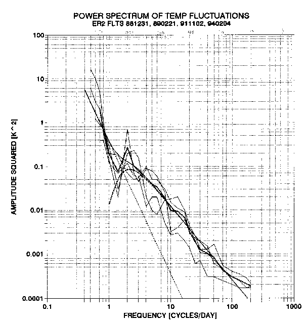From these data it is possible to decompose the spectrum of vertical motions of an air parcel travelling along the relatively unchanging isentrope surface, which can be associated with one particular streamline.  Figure 1 summarizes spectrae for four long, parallel-to-the-wind flights.  From this data it is apparent that invariably the wave amplitudes have a power spectral density that decreases with spatial frequency in accordance with a spectral index of -1.70 +/- 0.05.  This spectral index number is close to the theoretical prediction of -1.67, or -5/3.  The MTP data sample spatial frequencies between 0.6 and 200 cycles/day, which for typical wind speeds corresponds to wavelengths between 3000 km and 10 km, respectively.  Figure 1 shows a low amplitude feature at 1.4 cycles/day, which is bordered at the low frequency side by a steeply sloped rise of amplitude.  The low frequency portion of these spectrae are identified as the synoptic scale altitude displacements casued by low pressure and high pressure system disturbances to the vertical path of air parcel motion.  The synoptic scale vertical displacements are expected to have a spectral index of -3, which is compatible with the MTP data.

FIGURE 1 (apologies for this poor reproduction)

MTP observations also suggest that the amplitude of these waves increase with altitude, possibly according to the the reciprocal of the square-root of air density, which is the same relation found by the MTP for mountain waves. Although mesoscale waves obeying this spectral description are found at all locations and all seasons, the amplitude of the waves is greater over land than over ocean.  This implies that either orographic displacements of air flowing at the surface are amplified upward into the stratosphere, or the greater convection over land creates a rougher tropopause surface which causes greater vertical motions of lowermost stratospheric air flowing over the uneven troposphere boundary.  The amplitude of mesocale waves is also greater during winter than summer.  This may be related to the faster jet stream velocities during winter.

How Steep Slopes Might Trigger CAT

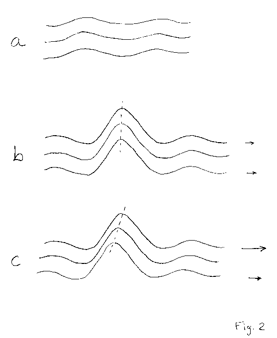
It will be useful to visualize the sequence of what might happen when a mesoscale atmopsheric wave grows to large amplitude because of the in phase addition of normal amplitude waves.  Figure 2a shows streamlines for a typical location before in phase wave addition.  The streamlines (i.e., isentrope surfaces) exhibit small vertical excursions that are approximately correlated with altitude.  Their amplitudes are approximately the same versus altitude, and their shapes are approximately aligned with altitude.  The displacement of a streamline from its mean altitude is typically 70 meters.   Figure 2b depicts a rogue wave without vertical wind shear; in other words, the large vertical displacements are aligned vertically, without horizontal phase shifts that accumulate with altitude.  Figure 2c has phase shifts produced by vertical wind shear.  The shift in phase with altitude defines a "phase line slope" and vertical wind shear produces a phase line slope that departs from vertical (designated by dotted lines in the figure).

To the extent that isotach surfaces and isentrope surfaces are displaced the same way streamlines are displaced, something can be said about changes in Richardson Number, Ri, for the cases in Fig.  2b and 2c.  In Fig. 2b Ri changes are small, whereas for Fig. 2c they can be large.  Since Ri has vertical gradient of wind squared in the denominator and vertical gradient of potential temperature to the first power in the numerator, Ri changes even when the two gradients change by the same ratio.  In Fig. 2b the two gradients remain unchanged, whereas in Fig. 2c they change.  The "leading edge," or upwind side of the rogue wave slope, has an increase of the two gradients.  This leads to a decrease in Ri, which brings Ri closer to the critical value below which the air is unstable.  When Ri decreases below 1/4, the air is unstable and CAT may be generated.

Can Rogue Waves Trigger CAT?

For rogue waves to be a significant trigger of CAT there must be a sufficient number of waves with steep slopes, and there must be sufficient vertical wind shear that the isotach and potential temperature surfaces are shifted with altitude sufficiently to change the vertical gradients of wind and potential temperature (causing Ri to decrease below 1/4).  A complete mesoscale atmospheric dynamical model would be needed to address this question, but it would still need to be initialized with a rogue wave having a realistic slope and phase line slope (which specify the change in Ri).

The remainder of this study is a first step in assessing the importance of rogue waves in CAT generation.  I will quantify how often large "rogue wave" slopes occur due to the "innocent" addition of normally occuring mesoscale waves.  It is hoped that follow-up studies will quantify how any pre-existing vertical wind shear will produce phase line slopes, and hence, how Ri will be affected by the rogue waves.

Approach

Isentrope surface altitude versus distance along a (stright line) hypothetical flight path will be constructed.  For each path a set of sine components will be added with random phases and amplitudes determined by a slightly noisy assignment of component amplitudes that are consistent with the spectral index of -5/3 and extending from spatial frequencies 2 to 256 cycles/day (1000 km to 8 km wavelengths).  Higher spatial frequencies probably exist, according to an interpretation of in situ temperature data, but they will produce slopes with horizontal extents  less than 2 km and correspondingly short longevities.  CAT generation requires long-lasting instabilities, at least several minutes, and large enough generating regions to extract sufficient energy to qualify as noticeable CAT.  I don't know where to place the threshold wavelength, so the results of this study will have to be qualified as applying to only "strong" CAT events, with the "strong threshold" left unspecified.

Each isentrope (i.e., streamline) trace that's created by adding all the sine components will be subjected to a "slope statistics" analysis.  This analysis will consist of a historgram of "numbers of events" with slope between specified values, with a histogram for each of several horizontal span lengths.  After many simulations a composite histogram will be produced for each span length.  The number of events will be converted to a "mean time between encounters" parameter, corresponding to a typical commercial airliner speed of Mach 0.75.  The outstanding events will be saved for display to show what an atmospheric "rogue wave" could look like - in terms of an isentrope cross-section.  From the knowledge of "mean time between CAT encounters" for the various levels of CAT severity the question can then be asked: Could a slope of magnitude such-and-so over a span of such-and-so generate CAT of a given magnitude?  The answer to these questions will then serve as input to an assessment of the merits of a further pursuit of the idea of rogue waves generating CAT, using, for example, dynamical meteorolgy tools.

Specification of Mesoscale Wave Amplitude Verus Spatial Frequency

The Y-axis in Figure 1 has units of Kelvin-squared.  The graph plots the square of the amplitude of spectral components that represent traces of temperature versus time for a specific potential temperature surface.  Since streamlines coincide with potential temperature surfaces these temperature changes correspond to vertical displacements of the specified surface.  The conversion is 9.7 K/km (assuming 19 km altitude, 40 degree latitude).  The X-axis is in units of "parcel time," which is the time required for a parcel to travel from the beginning of the measured data to the datum in question while travelling at 24 meters/second, which was the average wind speed for the flight under analysis (ER1991.11.02).

The data plotted in Figure 1 is averaged data, meaning that each point where line segments meet is the average amplitude of Fourier components (squared) for a range of spatial frequencies.  The range of spatial frequencies is proportional to the spatial frequency (i.e., has approximately the same apparent width on the graph).  An unaveraged spectrum for one flight is shown in Figure 3.   Note how well the -5/3 line fits the data.  This line has the equation A² =  f ^-5/3, where A is the amplitude of sine and cosine components [K] and f is spatial frequency [cycles/day].  If a spectrum of Fourier spatial components is constructed in accordance with the above -5/3 spectral relation, such that the sum of the squares of the sine and cosine amplitudes obeys the above relation, then the reconstructed trace of temperature versus time does not "look like" any observed trace.  It is therefore important to "add noise" to the spectral components if a realistic looking dT(t) trace is to be synthesized.

FIGURE 3

FIGURE 4

Figure 4 presents an example of a synthetic spectrum derived from an empirical algorithm that not only produces spectrae that look like the one in Figure 3, but also produce dT(t) traces that look like the one that is represented by Figure 3.  The equations incorporate a randomizing feature for producing Gaussian noise in specifiying the sine and cosine amplitudes.  The effect of this random Gaussian noise is to produce more negative noise than positive, and both negative and positive noise increases with spatial frequency (when noise perturbations are expressed as ratios).  These are apparently essential features for the proper synthesis of dT(t) traces.  The sine and cosine components for spatial frequency f, Asin(f) and Acos(f), are calculated from the following algorithm:

The sine and cosine components for spatial frequency f, Asin(f) and Acos(f), are calculated from an equation for their square:

Asin²(f) = R * f ^(-5/3)
    where R = 10^mX ... note, R ~ 1.0 since X ~ 0; R will range from slightly above 0.0 to maybe 2 or 3.
    X = -0.46 * Log_e(1/RND - 1)  ... this is a quick Gaussian function, returning + & - values with normal distribution having RMS = 1,
    m = 0.3 + 0.1 Log₁₀ (f) when X > 0,
    m = 1.2 + 0.5 Log₁₀ (f) when X < 0.

Spatial frequencies form a uniform sequence, f = 0.2775 [cycles/day] * N, where N = 1, 2, 3, ... 746 (i.e., f_max = 207.015 [cycles/day]).

To see the QuickBASIC program that creates Fourier components and then uses them to construct a dT(t) trace, click on ROGUE_BAS.

This is the correct way to represent a data sequence that is 1.8 days long represented by 745 values.  The data sequence actually consists of 2070 values, permitting components up to a maximum of 575 cycles/day to be included; however, excluding them is equivalent to low-pass filtering with a cut-off corresponding to the limit available for a data set with 4.9 minute sampling.  Inspecting the data indeed shows that the shortest spatial frequency is approximately the 7.0 minutes of parcel time that is expected from the use of a maximum spatial frequency of 207 cycles/day.  For an aircraft travelling at Mach 0.75, or 218 meters/second, the maximum spectral component of fluctuation represented by the synthesized data is 46 seconds.  The present analysis is therefore compatible with the goal of assessing the frequency of streamline slopes for distance spans of approximately 50 meters (or 14 seconds of aircraft travel time).  The set of Asin(f) and Acos(f), after performing the "noisy" adjustments, are used to straight-forwardly calculate a dT(t) trace, an example of which is shown in the next figure.

FIGURE 5

Figure 5 illustrates the reconstructed dT(t) trace (upper trace) and includes the measured data trace for the flight ER1991.11.02.  Note the similarity of "character."  Achieving this match in character was not easy, so it is important for anyone who wants to represent typical dT(t) traces that they use the equations given in the previous figure with only small adjustments to parameters.  The label "Synthetic 0" refers to the randomizing parameter the user enters my QuickBASIC program (ROGUE.BAS) which creates the syntheized traces.

Sample Output

The dT(t) traces have been imported to a QuattroPro spreadsheet, #ROGUE.WQ2, which was used to display and work with the statistics of "slopes" in the dZ(x), or altitude displacement versus distance trace, which was created by simple parameter conversions of the imported dT(t) trace.  Figure 6 is the Synthesis 0 trace of vertical displacement versus distance along flight path.

FIGURE 6

The 1-span slopes, corresponding to the slope acorss a 2.1 km span, are shown as a histogram in Figure 7. 
FIGURE 7

 The distribution appears "normal."  Figures 8 and 9 are the 2-span and 4-span slope histograms.  Again, there are no "outliers."

FIGURE 8

FIGURE 9

Figure 10 is a trace of the vertical displacement versus distance along "flight path" for a region that contains the highest and lowest points in the 4-span histogram (at x = 1220 and 1520 km).

FIGURE 10

It is interesting to note that if this were real data someone would be tempted to search for a meteorological explanation for these two steep slopes, while in truth they are merely the fortuitous adding and subtracting of a spectrum of normal, everpresent up and down air motions.

The previous analyses of synthetic vertical displacement traces are for one randomization choice simulation.  The "flight path" distance for this simulation is 4028 km, which corresponds to flight time of 5.1 hours (at Mach 0.75).  A similar analysis has been performed for 10 randomization choices, corresponding to 510 simulated flight hours.  The slope histograms for the 3 span distances exhibit Gaussian shapes with widths very similar to those in the above figures.  The steepest slope feature is shown in Figure 11.

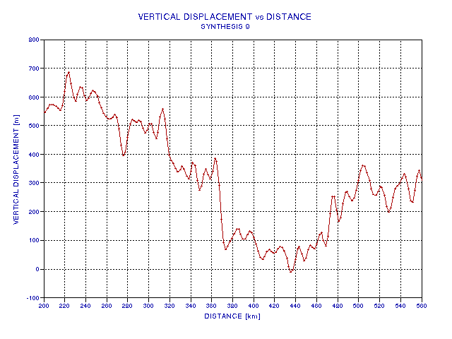
FIGURE 11

This feature is not what I imagined a rogue wave to look like, as it looks more like a cliff than an isolated wave.  In retrospect, this should have been expected when using "slope steepness" as the criterion for selection.  To produce a cliff we only require that several waves be aligned in phase at one location, whereas to produce a "pinnacle" type rogue wave would required that wave phases be aligned so that on one side of the wave the phases are aligned one way and on the other side of the wave theey're aligned the other way.

This simulation has shown that after about 500 flight hours, in air with waves similar to what is typically encountered at 19 km altitude, the steepest streamline slope that can be expected is 2.5 degrees (i.e., 280 meters over a span of 6.3 km).  For the ER-2 500 flight hours (at altitude) corresponds to about 10 flights.  During a typical 10 ER-2 flights it is likely that one "light to moderate" CAT encounter will be reported.  The next question is:  Will a 2.5-degree slope feature, accompanied by typical wind shear, exhibit sufficient instability to produce "rolling tubes" which will eventually generate "light to moderate" CAT?  This is a problem for a dynamical meteorologist.

Caveat

Rogue waves in the ocean may be produced by a physical phenomenon not represented by simply adding a normal spectrum of wave components using random phases.  If this is found to be true for ocean rogue waves, then it may also be true in the atmosphere.  However, rogue waves in the ocean are rare whereas CAT in the atmosphere is common, so unless a physical phenomenon that is rare in the ocean is common in the atmosphere this exotic explanation for ocean rogue waves would have little explanatory power for atmospheric CAT.

Concluding Remarks

Perhaps it was misleading to use the term "rogue waves" in the title for this study, since we do not yet know what causes them in the ocean.  This study, nevertheless, deals with the idea that wave components can add in unusual ways to produce an unusual surface topography, and the steep parts of such topographies might generate turbulence.  As far as I know this speculation is worthy of additional study, and the statistics on slope frequencies reported on here should be useful in future studies.

A side benefit of the present study has been the formulation of an algorithm for generating realistic traces of vertical displacement versus distance for the stratosphere.  Since vertical displacements produce temperature changes, and since these temperature fluctuations are important for some atmospheric chemistry problems, I have termed the ever-present waves described here as "mesoscale temperature fluctuations," or MTF.  The MTF amplitudes, after filtering out synoptic scale variations (using a spatial frequency cutoff of approximately 400 km), are surely smaller in the troposphere.  It remains to be determined if the same algorithm for simulating MTF in the stratosphere can be employed in the troposphere by merely reducing the wave component amplitudes, perhaps using the reciprocal of the square-root of air density as the correcting ratio.  If some CAT that is generated in the stratosphere turns out to be due to the rogue wave effect, it will be necessary to then determine if the same proportion of tropopsheric CAT can be explained the same way.

The next step in pursuing the idea that rogue waves generate CAT is to employ mesoscale dynamical atmospheric models to simulate 2 to 3 degree slopes under a variety of vertical wind shear conditions.

PostScript:

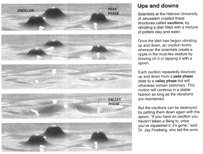
The following is part of an article that describes the laboratory production of what they call "oscillons" that are caused by reflections off boundaries in a medium that is subject to vibrations.  The authors believe the oscillon concept can be applied to the way earthquakes can produce spotty damage.  I wonder if mountain ranges can "reflect" waves and also produce in-phase atmospheric coounterparts to oscillons.

This article appeared in the Santa Barbara News-Press, 199 October 12.
 

____________________________________________________________________

This site opened:  May 8, 1999.  Last Update: October 13, 1999