
Bruce L. Gary
Jet Propulsion Laboratory, Pasadena, CA
Abstract
Synoptic scale assimilations of radiosonde and satellite data for the global temperature and wind fields are limited to spatial wavelengths longer than about 400 km. The assimilated wind field is frequently used to calculate back trajectories, and the temperature field is then used to calculate histories of air parcel temperature. Reliance upon assimilated data for back trajectory temperatures has the following shortcomings: 1) the absence of mesoscale features means that their associated short timescale temperature fluctuations are not present, and 2) errors in the synoptic data can cause significant errors in the synoptic component of temperature histories. The airborne Microwave Temperature Profiler measures the temperature field within an altitude/ground track cross-section, and this provides an ideal means for evaluating the magnitude of both error sources.
It is found that the first shortcoming of back trajectory temperatures, the lack of mesoscale temperature fluctuations, is greatest over land, especially mountainous topography, and is smallest over mid-latitude and high-latitude oceans. A seasonal effect is also present, with winter producing greater fluctuations. The amplitude of mesoscale fluctuations increase with altitude in way that is similar to that for mountain waves. A stochastic algorithm has been derived for simulating mesoscale temperature fluctuations, and this component of fluctuation can be added to back trajectory temperature sequences for the purpose of evaluating the implications of the first shortcoming category.
The second shortcoming of back trajectory temperatures, assimilation data base errors, can produce synoptic scale variations of several degrees K. Temperature offsets of as much as 3 K can persist for more than a day of parcel time. Additional cases must be studied before this component can be simulated using stochastic algorithms.
"I wouldn't have seen it if I hadn't believed it!" (An old geologist saying.)
Observationalists have a tradition of creating new tools for viewing nature. When an instrument opens a new "observational window" it invariably discovers new things which force theoreticians to revise, or at least refine, their models. The airborne Microwave Temperature Profiler, MTP, developed at Caltech's Jet Propulsion Laboratory, is such an instrument. One of its most significant and unexpected findings, though in retrospect it should have been anticipated, is the existence of an ever-present structure of altitude displacements of isentrope surfaces, implying the presence of corresponding temperature fluctuations for air parcels travelling along isentropes.
It is inevitable that the 3-D temperature field has more structure than is represented by assimilated data fields. The input to an assimilation model consists of radiosonde profiles and satellite measurements, and the sampling locations for these sources of data are too sparse to capture small scale spatial structure. Even if satellite data contained a complete representation of 3-D structure it would have to be smoothed to be consistent with the finite horizontal and vertical node spacing of assimilation models.
In 1987 the MTP made measurements from a NASA ER-2 aircraft during the Airborne Antarctic Ozone Experiment. MTP data for the flight of 1987 September 22 was used to construct the first airborne "isentrope altitude cross-section," or IAC, from a single aircraft flight segment. By a happy coincidence this first IAC showed an atmospheric mountain wave (Gary, 1989) so large that a larger one was not observed with the MTP for another 960 flight hours, when on January 22, 2000 an even larger mountain wave was encountered (Mahoney, private communication). Gary (1989) and Bacmeister and Gary (1989) have used MTP data to show that the amplitude of short spatial wavelength variations of isentrope altitude is greater during flight over land than over ocean, at least at polar latitudes and during winter.
In 1989, during the Airborne Arctic Stratospheric Experiment II, the MTP was included on the payload of a NASA ER-2 aircraft. These arctic flights showed a similar pattern of mesoscale structure, but this time it got the attention of modelers trying to reconstruct parcel temperature histories along back trajectories. The fluctuations of air parcel temperature required by the mesoscale isentrope structures represented a potential concern to modelers who required accurate representations of air parcel temperature histories being used to infer temperature-sensitive changes to aerosol chemistry and denitrification of the winter polar vortex. Isentrope surface altitudes from an MTP IAC had far more structure than was produced by traditional back trajectory calculations. Some modelers were reluctant to believe that the MTP-measured mesoscale structure was real, perhaps motivated by the recognition that such structure would require longer computer runs for trajectories that incorporated mesoscale temperature fluctuations. Studies began "in the field" to evaluate the implications of superimposing the MTP-required mesoscale temperature fluctuations onto back trajectory temperature histories (Wofsy et al, 1990). A few years later, Murphy and Gary (1995), and Tabazedeh et al (1996), also explored implications of this new component of temperature structure.
The MTP is an ideal instrument for evaluating the magnitude of errors in an assimilated temperature field. No other instrument directly measures properties required for determining isentrope altitudes. The MTP-derived temperature profiles, and the isentrope altitudes that are derived from them, provide for spatial resolutions of approximately 3 km along a flight track. The magnuitude of errors in an assimilated temperature field can be evaluated by comparing MTP measured IACs with IACs prepared from synoptic temperature fields using "assimilated" data. An example of such a comparison is presented in the next section.
Modelers who would like to evaluate the implications of omitting the mesoscale component of temperature fluctuations in their back trajectory temperature calculations due to both assimilated field errors and mesoscale temperature fluctuations will find guidance for performing these analyses in a later section of the article. Investigators relying upon back trajectories should consider performing a series of stochastic back trajectory calculations for the purpose of probing possible implications of realistic temperature histories similar to the one the air parcel in fact experienced.
A future publication will present a quantitative analysis of Mesoscale Fluctuation Amplitudes (MFA) for many regions, seasons, underlying topography and altitudes. Equations, and a table, summarize the dependence of MFA upon these four independent variables. This article presents a table of typical MFA for a variety of settings, and an equation representing altitude dependence allows for the prediction of a "most likely MFA" for any altitude with categories of latitude, season and underlying topography.
There is a tendency for things "out of sight" to be "out of mind." Some investigators who only occasionally use synoptic-scale data have apparently been lulled into thinking that mesoscale temperature structures don't exist. "After all," goes the unconscious thinking, "it never shows up in assimilation temperature fields." Other investigators readily acknowledge that mesoscale fluctuations exist, but believe they are negligible for most model analyses. Any neglect of a known effect carries with it a "burden of proof" for the investigator to at least demonstrate that for the category to which the specific case belongs the effect may be ignored with no consequence to the eventual conclusions of the investigation.
This article presents "the case" for the existence of mesoscale structures in the atmospheric temperature field, and quantifies the structure in the temperature field that is missing in synoptic scale (assimilation model) representations.
2. Mesoscale Versus Synoptic Scale Temperature Field Structures
Figure 1. An example of a typical synoptic scale "isentrope altitude cross-section," or IAC. It shows the altitude of potential temperature surfaces versus latitude along a ground track flown by NASA's ER-2 aircraft on March 27, 1994.
This figure is based on a 3-dimensional field of assimilated data, derived from radiosonde and satellite temperature measurements. This IAC presentation was calculated from an XS-file produced by Schoeberl, Newman, Nagatani and Lait of the NASA Goddard Space Flight Center (1994), which in turn was constructed by sampling a 3-dimensional assimilated temperature field based on radiosondes and satellites. This data is in the "public domain" in the form of compact disks issued at the completion of the ASHOE/MAESA mission, and also on a computer at NASA's Ames Research Center used to maintain an archive of airborne data taken with Ames Research Center science platform aircraft (now at Dryden Flight Research Center). This data, as well as other data for this date, were taken as a part of a NASA-sponsored mission called "Airborne Southern Hemisphere Ozone Experiment/Measurement for Assessing the Effects of Stratospheric Aircraft" (ASHOE/MAESA).
The isentropes in the figure are for stratospheric air (the tropopause is at about 16 km) along a flight track "curtain" cross-section oriented approximately north-south. Although the wind direction for this data is "out of the page," it can nevertheless be used to estimate the values of isentrope slopes in an orthogonal (parallel to the wind) cross-section, since cross-sections at a given location typically exhibit isentropes with a similar "wrinkle character" in cross-sections of all azimuths, provided mountain waves are not present (Gary, unpublished). Thus, from this figure it can be said that air parcels following isentrope surfaces rise and fall approximately 100 meters, with periods corresponding to spatial wavelengths of about 900 km (8 arc degrees). The Meteorology Measurement System, MMS, (Chan et al, 1994) measured the wind speed in this region to be 10 m/s, eastward, so we may conclude that an air parcel's altitude variations produced temperature fluctuations that were typically 1 K with periods of 25 hours. Heating and cooling rates for such air parcels is of the order of 2 or 3 K/day. Trajectory analyses based on assimilated data for this region would therefore produce relatively benign heating and cooling rates and small temperature changes on 1-day time scales.
The airborne MTP instrument measures an altitude profile of temperature every 10 seconds (for 1994 data). This corresponds to 2.1 km (or 0.02 degrees of latitude for north/south flight). Each T(z) profile extends from approximately 4 km below flight altitude to 4 km above. Figure 2 shows isentrope altitudes derived from MTP measurements for the same flight track as in the previous figure. The MTP-measured IAC in Fig. 2 appears to have short spatial scale structure that does not exist in Fig. 1.
The two cross-sections are overlayed in Fig. 3, and it shows dramatic differences between the assimilated and MTP-measured temperature fields. Assuming the MTP-based IAC is correct (as argued below), the differences reveal that a significant amount of mesoscale structure exists which is not captured by the synoptic scale assimilation. This comparison also shows the presence of small errors in the assimilated temperature field. Near flight level, for example, the RMS difference between the two isentrope altitudes is 170 meters, and the maximum difference is 390 meters. It is also apparent that the highest spatial frequencies in the synoptic plots are misleading, which is to say that about half the time the small structures in the synoptic isentropes do NOT correlate with features in the measured isentropes.
How much credibility is there for the isentrope differences between MTP and the synoptic data? The shortest answer to this question is to cite the fact that there is always good agreement between MTP's temperature profile value at flight level and the MMS in situ air temperature record. When the MMS 1 Hz data is smoothed to correspond to the slower sampling of the MTP, the two temperature traces agree to within approximately 0.3 K, and there is even better agreement for the variations over time (i.e., small offsets may exist, but the shapes are essentially identical). This provides assurance that the MTP isentropes near flight altitudes are accurate, and that their up and down variations are correct. Near flight altitude the variation of isentrope altitude is accurate to approximately 35 meters.
Comparisons have been made of MTP measurements with radiosonde-based predictions of what MTP should measure for times when the aircraft flies close to radiosonde sites. Based on these comparisons it is estimated that MTP's temperature profile of RMS accuracy is less than 1.0 K for a 3 km altitude region centered upon flight altitude, and that at the extremities of an 8 km region (centered upon flight altitude) the RMS accuracy of MTP T(z) profiles is approximately 2.5 K. Therefore, for isothermal stratospheric flight, for example, MTP temperature profiles can be used to determine isentrope altitudes with an accuracy of 100 meters near flight altitude, 250 meters at 4 km above and below flight altitude, and intermediate accuracies values between these altitudes. (For typical polar ozone conditions, with dT/dZ = -2 K/km, the isentrope altitude accuracies are 130 meters and 320 meters.)
Since precision is always better than accuracy, assuming calibration errors vary slower than measurement intervals, the altitude structure of isentropes is better than would be implied by the accuracies just quoted. It is reasonable to adopt the 35 meter accuracy for isentrope altitude structure near flight altitude, derived from comparisons with MMS, and to adopt 100 meters precision for structures at 4 km above and below flight altitude. These precision estimates are compatible with known stochastic measurement uncertainties.
The implication of the analyses of MTP accuracy and precision is that essentially all of the structure differences in Fig. 3 are statistically significant and are therefore real.
The previous isentopre "behavior" was at tropical latitudes, using data from the 2-channel ER-2 MTP. The next example covers a latitude region from Hawaii to Alaska, and the MTP used was a more modern design, 3-channel version mounted on the NASA DC-8 aircraft and flown during 1995/96 flights for TOTE/VOTE (Tropical Ozone Transport Experiment/Vortex Ozone Transport Experiment).
The measured isentrope altitude cross-section in Fig. 4 shows much more structure than the assimilated version. In particular, a sub-polar jet has distorted the isentrope field at about 53 degrees north latitude, at 10.5 km. Also, the sub-tropical jet has produced steeper isentrope surfaces at 35 north latitude, at 10 to 12 km altitude. This figure shows that not only are isentrope shapes much more interesting in the real world, but assimilated isentrope altitudes can be in error by as much as 900 meters (e.g., 51 degrees north latitude, 10 to 11 km, and also at 21 degrees latitude, 12 to 16 km). The effect on isentropes of the sub-tropical jet, located at 35 degrees north and 10.4 km, is dramatic in the MTP data, but subdued in the assimilation data.
Figure 5 is a color-coded display of the MTP temperature field from which the previous IAC was determined. In the vicinity of the sub-polar jet in situ tracer measurements were used to define the tracer tropopause (ozone mixing ratio of 100 ppbv), and there is corroboration that the temperature field is distorted at the same location as the tracer field. In the vicinity of the sub-tropical jet both in situ and remote tracers are used to define the tracer tropopause. The Langley DIAL ozone profiler (Browell, E. V., 1989) determined isopleths of ozone mixing ratio, which have been used to define the "tracer tropopause" above the aircraft south of 36 degrees north latitude. By combining in situ and remote tracers it was possible to derive a very steep slope for the tracer tropopause at 38 degrees latitude, just poleward of the jet.
All of the tracer tropopause behaviors found in this figure are consistent with the expected circulation of air in the vicinity of jets. The black arrows are a subjective suggestion of a "residual circulation" pattern that could produce the temperature departures from a smoother version, and it is compatible with conventional models. A more complete description of this flight (unpublished) is available from the author. The purpose in presenting this figure here is to support the MTP version of the isentrope field as providing accurate mesoscale temperature field structure that is missing in assimilated temperature fields.
3. Measured Temperature Fluctuations for a Single Isentrope
Figure 6 shows a different method for studying isentrope structure, and it is based on a ER-2 MTP measurements at mid-latitudes. This figure shows the altitude of a single isentrope. Since vertical displacements imply adiabatic temperature changes, this data shows that reliance upon assimilated (synoptic) temperature field data for deriving time histories of temperature for an air parcel will underestimate the extent of actual temperature variations. Since in this case the synoptic trace was derived by smoothing the measured trace, temperature differences will not include errors that would be present if an actual back trajectory temperature trace were used. This method for deriving the mesoscale component of temperature fluctuations therefore produces underestimates of differences between "true" and "assimilation field" for a back trajectory temperature calculation.
During this flight the ER-2 encountered a constant wind of 24 m/s moving generally eastward, parallel to the direction of flight. Since an air parcel will follow an isentrope surface (provided diabatic heat exchange rates are small) the 490 K isentrope can be used to infer air parcel's temperature fluctuations. The figure shows how an air parcel, traveling along the 490 K isentrope, would change temperature if the 490 K isentrope surface did not change shape during the parcel's 2-day trip. It doesn't matter that we don't know how the isentrope surface changed during any 2-day period of a hypothetical parcel trajectory since we are only interested in a qualitative assessment of the importance of neglecting mesoscale structures when calculating parcel temperature histories. A qualitative answer for this "real atmosphere" setting, chosen at random, is shown by the "difference temperature" trace in Fig. 7.
Figure 8 shows that the mesoscale versus synoptic scale temperature differences can be fitted by a Gaussian, and for this case the Gaussian's "full-width at half-maximum" is 1.6 K. This article uses a "full-width at half-maximum" parameter to represent the "mesoscale fluctuation amplitude," or MFA. Thus, MFA = "full-width at half-maximum" of the mesoscale-only temperature fluctuation histogram.
There are several practical ways to derive MFA. It can be quickly estimated from a data sample by drawing a smooth line through a measured isentrope surface's altitude versus distance (omitting all spatial components with wavelengths shorter than about 400 km), then counting or estimating a "probable error (PE) difference" such that 50% of actual data exceed this probable difference. This PE value should be multiplied by 3.33 to arrive at the "full-width half-maximum" estimate. To convert this MFA from altitude units to temperature, divide by 100 meters/K (since every 100 meter altitude displacement corresponds to ~1 K of temperature change, corresponding to the adiabatic lapse rate of dry air).
An MFA estimate can also be obtained by noting that 76% of all data will be contained within the upper and lower MFA boundaries. Or, for one more alternative method, MFA can be computed by multiplying an RMS difference by 2.27 (an RMS can be estimated from the fact that in a normal distribution 68% of deviations will have an absolute value less than the RMS; the factor 2.27 has been empirically determined for MTP data, and is close to the value 2.36 that corresponds to a perfect Gaussian distribution). Section 5 includes a table of MFA values for a variety of location and season settings.
4. Assimilated versus Measured Single Isentrope Offset
Fig. 9 shows the same 490 K isentrope described in the previous section, but it includes for comparison the 490 K isentrope altitude derived from an assimilated data base (as archived in the XS-file for AASE2). The difference between "true" and "assimilated" parcel temperature versus parcel time is presented in Fig. 10. The two shortcomings of using an assimilated field for calculating parcel temperature is apparent in this figure: 1) the assimilated field has an offset error, and 2) it lacks short wavelength spatial components for an isentrope's altitude. The assimilated trace has an offset that ranges from ~0.2 km to ~0.4 km (i.e., 2.0 K to 4.0 K).
For the case of the ER-2 flight of 1991 November 2 (chosen for convenience and not because it was thought to be unusually discrepant with assimilation data), the histogram of "back trajectory air parcel temperature differences" derived by comparing MTP-measurements with archived synoptic data is shown as Fig. 11. The best way to "understand" this histogram is to remember that it consists of two components: 1) a quasi-stochastic component (Gaussian), and 2) an offset component, which will vary gradually with location (i.e., parcel time). The stochastic component is associated with "mesoscale temperature fluctuations," and has a characteristic "width" that will depend on altitude, latitude, season and underlying topography. The offset component is associated with assimilation errors, and will vary slowly, wandering on both sides of zero (presumably). The offset component is likely to be larger over the ocean, or wherever radiosondes are sparse (and only satellite or ship soundings are available). Figures 1 to 3 suggest that this component may be larger in the tropics, where assimilation models have trouble constraining solutions (reference needed).
The Fig. 8 discussion employed MFA (mesoscale fluctuation amplitude) to represent a Gaussian fit's "full-width at half-maximum." Whereas Fig. 8 has MFA = 1.6 K, the same data when compared with an actual archived synoptic data base shows differences with an MFA of 2.4 K. Figure 8 was merely showing the presence of a stochastic term and neglected wandering offset errors. Any attempt to estimate the RMS error of trajectory temperatures based on synoptic data must deal with an unknown and varying offset, which in the case just described was 3.2 K. (Recall that the procedure for deriving Fig. 8 assured that it would have no offset.) Since the contribution of mesoscale fluctuation variations to the observed spread in Fig. 11 has been determined to be 1.6 K, it is possible to determine the contribution to Fig. 11's spread due to "assimilation error wander." The orthogonal subtraction of 1.6 K from 2.4 K gives 1.8 K, and this must be the wander variation of assimilation error for the 2-day parcel trajectory for the case study.
The present analysis characterizes the contribution of shortcomings of the assimilated data base to the back trajectory temperature history that would be calculated for an air parcel found above Maine, at the 490 K surface, on 1991 November 2 just before the ER-2 descended to land. It will be useful to name the two parameters that characterize this variation, which follows:
Table I. Parameters Describing Assimilation
Temperature Field Errors in Back
Trajectory Calculations for the Specific MTP ER-2
Case Study
| Trajectory Temperature Error Offset | 3.2 K for 1991.11.02 (2-day parcel time) |
| Trajectory Temperature Error Variations | 1.8 K for same data |
| Missing Mesoscale Component | 1.6 K for same data |
With the analysis of more cases it should be possible to represent the character of trajectory temperature histories by employing an algorithm that creates simulated trajectory temperature histories associated with the first two error types listed above, the "Trajectory Error Offset" and "Trajectory Error Variation." The goal for such a study would be to provide a method of creating simulated trajectory temperature histories using a stochastic procedure for representing simulated mesoscale temperature fluctuations. When this has been achieved (it is beyond the scope of this investigation) it will then be possible to calculate a series of simulated dT(t) series for superimposing on back trajectories calculated from assimilated fields T(t) to arrive at a more realistic set of hypothetical T'(t) series that hopefully would provide a more realistic set of histories that the parcel under study actually underwent. Such a set of hypothetical T'(t) could then be used as input for evaluation by models that calculate other things, such as the likelihood of cloud formation, or the amount of a chemical reaction that is very temperature dependent.
Figure 12 may be helpful in visualizing the distinction between slow "trajectory temperature variations" and the faster "mesoscale temperature fluctuations," all of which must be combined for deriving dT(t) series to be used in simulating the effects of temperature variations not captured by a back trajectory temperature sequence. This figure shows the slowly varying component of error in back trajectory temperature history due to assimilation data base errors using a smooth trace, whereas the faster mesoscale temperature fluctuations are represented by histograms. Both components must be combined to arrive at a simulation of a temperature history error trace, dT(t), that should be superimposed upon a back trajectory temperature trace that is based on synoptic data. Since the magnitude of both components are not known, they must be constructed using stochastic algorithms, and many such constructed dT(t) series must be added to the "reference" back trajectory T(t) to evaluate the magnitude of effects that can be attributed to the unknown temperature variations.
For a specified interval of time (such as the first half of Fig. 12), the two components produce unkown errors that can be described by 1) an offset with a wandering amplitude, and 2) faster varying mesoscale fluctuations. As described above, for the ER-2 flight of 1991 November 2, these three errors had values of 3.2 K, 1.8 K and 1.6 K.
A goal for future work is to fabricate stochastic algorithms that adequately represent the offset error temperature variations. A procedure for constructing realistic mesoscale temperature fluctuations is available from the author. Analyses to date comparing MTP-derived isentropes with assimilated isentropes is insufficient to permit a derivation of stochastic algorithms for representing the "wandering offset error" component.
5. Spectral Properties of Mesoscale Temperature Fluctuations
In order to understand the origin of the mesoscale isentrope wrinkles, which produce temperature fluctuations for constant altitude flight, it will be useful to investigate their spatial spectrae. Figure 13 is a spectral energy density spectrum for one flight and a specific isentrope surface. Since the wind speed was an almost constant 24 m/s during the flight (parallel to the flight direction), it was possible to convert ground track distance to parcel time, allowing for the spectrum to be presented in terms of "cycles per day." A few spatial wavelengths have been noted at the top of the graph. The well-known synoptic spectral index of -3 has been fitted to the long spatial wavelength data. A mesoscale component having a high spatial frequency spectral index of -5/3 has been fitted to the higher frequency data (shorter spatial wavelengths). This component has a rounded long spatial wavelength "termination" that was arbitrarily chosen to provide a good fit of the sum of the two components to the measurements for this and other flights.
The spectrum at high frequencies appears to "level off" for frequencies higher than about 200 cycles/day. Since the MTP instrument measures oxygen emission from a distance of a few kilometers, this type of high frequency feature is expected. A similar analysis was performed on an IAC produced from 1 Hz MMS data (using lapse rates from MTP) and the high frequency "leveling off" does not occur with that spectrum at the same spatial frequency. Presumably, the spectrum of isentrope fluctuations continues to decrease with a slope of -5/3 for frequencies higher than those sampled here.
Three other MTP/ER2 data sets with long flight segments parallel to the wind were subjected to the same spectral analysis, and in every case the same pattern was present, namely: 1) a synoptic scale component was present for frequencies below 1.5 cycles/day and having a slope of about -3, 2) there's a local maximum in spectral power at about 2 cycles/day, and 3) for frequencies higher than ~2 cycles/day the spectrum exhibits a slope of about -5/3. The average spectrum for these flights is shown in Fig. 14.
The spectral feature at 1.5 cycles/day might be produced by an atmospheric tides explanation, which would predict such a feature (invoking 2 cycles/day as a "source" frequency). "Windowing" of the data was performed, as is necessary for any finite data set before it can be subjected to a power spectrum analysis. It is unlikely that windowing could produce a "dip" structure at the same frequency when wind speeds differed for the several flights. This 1.5 cycles/day feature remains unexplained.
The best fit slope for the 3 to 100 cycels/day region is -1.70 +/- 0.04. This is statistically compatible with -5/3 (i.e., -1.67). Nastrom and Gage (1985) published a classic analysis of temperature fluctuations from commercial aircraft, and they found it necessary to invoke a transition from a slope of -3 at synoptic scales to -5/3 at mesoscales. Their transition region was at about 2 or 3 cycles/day. The Nastrom and Gage spectrum is shown in Fig. 14. It was not apparent how to convert their spectral density scale to the one used in this analysis, so a vertical shift was applied to the Nastrom and Gage spectrum in order to achieve agreement between the two synoptic scale portions. This method for comparing the spectrae for the two data sets is equivalent to assuming that over the range of synoptic scale spatial frequencies the amplitude (and spectral index) for large samples of data are the same over the altitude region 10 to 20 km, whereas the mesocsale component may vary with altitude. If this assumption is correct, then the fact that the ER-2 mesoscale spectral componenet is greater than the Nastrom and Gage mesoscale spectrum component implies that mesoscale fluctuations increase with altitude. This is not only reasonable, but is supported by MTP/DC8 data, to be described next.
Isentropes are more wrinkled at ER-2 altitudes than at DC-8 altitudes (in preparation), where it is shown that MFA_ER2 is 1.64 times greater than MFA_DC8. Mountain wave theory predicts a ratio of 1.88 for moutain wave amplitudes. Gary (1989) shows that mountain wave amplitude increases with altitude in accordance with mountain wave theory, with MFA being proportional to the reciprocal of the square-root of air density (which preserves wave motion energy with altitude). If the typical altitude of the aircraft in the Nastrom and Gage study is the same as for the DC-8 (11.4 km), and if the mix of stratospheric and tropospheric flying is the same for the DC-8 and Nastrom and Gage data sets, then at ER-2 altitudes the mesoscale altitude excursions should be 1.64 times greater than the Nastrom and Gage excursions. In other words, the spectral energy, which is proportional to the square of the amplitude, is predicted to be 2.7 times greater at ER-2 altitudes compared with commercial flight altitudes. In Figure 14 the two amplitudes appear to be have a ratio of 5 or 6, which is about twice the expected value.
The Nastrom and Gage data set is for flight at mostly mid-latitudes, it is for all seasons, and occurs over a typical mix of topographies, whereas the DC-8 MTP data are mostly in winter, high latitude (for study of the "ozone hole"). If the Nastrom and Gage flights are assumed to be at an average altitude of 11.0 km (36,000 ft), during all seasons, at 40 degrees latitude, and over the same topography as the DC-8, the MFA model developed from MTP data on the of the ER-2 and DC-8 (in preparation) predicts an MFA ratio of 1.46, and a spectral energy ratio of 2.14. This additional correction is exactly what is needed to reconcile the 5 or 7 times greater spectral energy shown in Fig. 14 (i.e., 2.7 times 2.14 = 5.8). Therefore, the Nastrom and Gage data, as presented in Fig. 14, is compatible with the ER-2 MFA data.
These several MFA properties can hopefully be used by atmospheric scientists to formulate an underlying theory for the origin of mesoscale isentrope wrinkles.
6. MFA Statistics
As described elsewhere (in preparation), MTP data have been used to derive an equation for predicting Mesoscale Fluctuation Amplitude, MFA. Segments of 91 DC-8 and ER-2 flights were subjected to an identical analysis that yielded MFA estimates for an assortment of latitude, season and underlying topography. Since the DC-8 and ER-2 flew at very different altitudes (11.4 and 19.4 km), it was possible to include air pressure as an independent variable. A least squares regression analysis was performed using many possible independent variables, and it was determined that these four variables had statistically significant correlations to warrant inclusion in a model for predicting MFA: season, latitude, underlying topography and altitude. The MFA model is a first-order model for representing MFA values over a wide altitude region, seasons, latitudes and topographies, and a purpose of this article is to suggest that its use as a better alternative to a total disregard of the MFA effect.
The following table of MFA values is based on the preceding analysis, and may be convenient for casual users wishing to estimate the possible importance of the MFA effect. To use the table, choose a latitude region (left-most column), choose a season (center two columns), and choose an underlying terrain (right-most column), and note the MFA listed in the body of the table. This MFA is what can be expected at ER-2 altitudes (19.58 km); for DC-8 altitudes, for example, multiply the MFA value by 0.59. For other altitudes, multiply the MFA value by (58.5[mb] / P[mb])0.41.
TABLE 2 - MFA for ER-2 Altitudes (19.58 km)
(Multiply by 0.59 for DC-8 Altitudes, 11.44 km)
| Latitude Region | WINTER | SUMMER | Underlying Terrain |
| POLAR | 239 meters
186 " |
68 meters
16 " |
Mountains
Ocean |
| MID-LATITUDE | 173 meters
121 " |
125 meters
72 " |
Mountains
Ocean |
| TROPICAL | 176 meters
124 " |
173 meters
120 " |
Mountains
Ocean |
There is a large range of MFA values typical for the various settings, especially for the polar regions. For example, "Polar/Summer/Ocean" exhibits MFA = 16 meters, whereas "Polar/Winter/Mountains" exhibits MFA = 239 meters! It is unsurprising that there is very little seasonal effect of MFA in the tropics, since the tropics experience only modest changes in weather versus season. Likewise, it is unsurprising that the polar region undergoes a greater seasonal variation than the other latitude regions. Patterns like these may be viewed as indirect confirmation of the quality of the original measurements.
Due to space limitations, it is not possible to include a description here of the algorithm for creating simulated, stochastic mesoscale fluctuations dT(t) for superimposition upon synoptic scale back trajectory temperature histories; the algorithm is available from the author. Back trajectory investigators may want to devise their own slgorithms, based on the qualitative appearance of measurements presented in this article. Assuming that a stochastic dT(t) function is available, and that it has a standard RMS deviation of 1 K, a specific dT(t) sequence for adding to a back trajectory can be derived by multiplying this nominal 100 meter amplitude MFA dT(t) sequence by the ratio of the desired MFA (from the table, above) to 100 meters. As an alternative to using a reference 100 meter MFA dT(t) algorithm, the user may request from the author sequences of dT(x) already prepared that exhibit MFA of 100 meters, and then: 1) convert the distance coordinate, x, to time by assuming a parcel velocity, and 2) multiply the dT(t) function just derived by the ratio (MFA_desired) / (100 meters).
If a specific dT(t) function is not required, but a probability density distribution for dT is adequate, then this can be easily calculated from P(dT) = EXP((-dT/0.60*MFA)2), which is normalized such that P(0) = 1. MFA is first calculated from the MFA Table 2.
7. MFA Origins
The MFA equation suggests that mesoscale fluctuations originate with surface topography. This suspicion is supported by noting that in Table I, where 6 comparisons of "mountains versus ocean" are presented the greater MFA is associated with mountains. Of course, topography cannot by itself produce vertical displacements; the wind is also a requirement. Winds are stronger in the winter (due to the greater latitude gradient of heating then), so if mesoscale fluctuations are produced by winds encountering surface topography MFA should be larger for the winter season. Indeed, this is the case for all 6 comparisons in Table 2.
The fact that MFA increases with altitude merely favors the fact that the mesoscale fluctuations originate below DC-8 flight altitudes, which is consistent with.the topography/wind speculation. It is significant that in the tropics mesoscale fluctuations are present at DC-8 altitudes, which probably rules out the tropopause as a source altitude (since the DC-8 is always below the tropopause when flying in the tropics). Perhaps overshooting turrets produce a form of orography from the standpoint of winds near the tropopause, and perhaps a theory could be constructed that places the generation of mesoscale fluctuations at the tropopause with propagation both upward and downward. However, such a theory could not account for the observed correlation of MFA with surface topography in the tropics.
The measurements reported here constitute a strong case for placing the altitude of origin of mesoscale fluctuations at ground level, with low altitude winds having to undergo vertical motions as they follow topographic relief. Since mesoscale fluctuations are present everywhere, at all times, it could be asserted that the atmosphere is in an ever-present state of excitement by mountain wave motion.
Acknowlegements
The research described in this paper was carried out by the Jet Propulsion
Laboratory, California Institute of Technology, under a contract with the
National Aeronautics and Space Administration. Specific acknowledgement
is made for the contributions of Richard Denning for his instrument expertise
throughout all field uses of all Microwave Temperature Profilers, and to
Dr. M. J. Mahoney whose encouragement helped bring this work to publication.
Appreciation for the use of ozone data produced by Dr. Edward Browell's
DIAL team is hereby acknowledged, as is Meteorology Measurement System
in situ data produced by a team headed by Dr. Roland Chan.
REFERENCES
Bacmeister, J. T. and B. L. Gary, 1990, "Small-Scale Waves Encountered During AASE," Geophys. Res. Lett., 17, 349-352.
Browell, E. V., "Differential Absorption Lidar Sensing of Ozone," Proc. IEEE, 77 , 419-432, 1989.
Gary, B. L. 1989, "Observational Results Using the Microwave Temperature ProfilerDuring the Airborne Antarctic Ozone Experiment," J. Geophys. Res., 94, 11223-11231.
Murphy, D. M. and B. L. Gary, 1995, "Mesoscale Temperature Fluctuations and Polar Stratospehric Clouds," J. Atmos. Sciences, 52, 1753-1760.
Nastrom, G. D. and K. S. Gage, 1985, "A Climatology of Atmospheric Wave Number Spectra Observed by Commercial Aircraft," J. Atmos. Sci., 42, 950-960.
Tabazadeh, A., O. B. Toon, B. L. Gary, J. T. Bacmeister and M. R. Schoberl, 1996, "Observational Constraints on the Formation of Type Ia Polar Stratospheric Clouds," Geophys. Res. Lett., 23, 2109-2112.
Wofsy, S. C., G. P. Gobbi, R. Salawich and M. B. McElroy, 1993, "Vapor Pressure of Solid Hydrates of Nitric Acid: Implications for Polar Stratospheric Clouds," Science, 259, 71-74.
Wu, D. L. and J. W. Waters, 1996, "Gravity-Wave-Scale Temperature Fluctuations Seen by the UARS MLS," Geophys. Res. Lett., 23, 3289-3292.
Wu, D. L. and J. W. Waters, 1996, "Satellite Observations of Atmospheric Variances: A Possible Indiocation of Gravity Waves," Geophys. Res. Lett., 23, 3631-3634.
FIGURES AND CAPTIONS

Figure 1. Isentrope altitude cross-section, based on assimilation
data, for the ER-2 flight of 1994 March 27, from Fiji to New Zealand. The
isentropes are 10 K of potential temperature apart,
starting with 430 K (at about 17.3 km). The ER-2's altitude is
shown by the thin black trace.

Figure 2. Measured isentrope altitude cross-section using the 2-channel MTP/ER2 instrument for the same period as Fig. 1.

Figure 3. Overlay of Fig.'s 1 and 2, showing the difference between mesoscale (green and blue) and synoptic scale (red) isentropes.

Figure 4. Overlay of assimilated (red) and measured (green and blue) isentrope altitude cross-sections for a DC-8 flight from Alaska to Hawaii on December 11, 1995. The isentropes are 10 K of potential temperature apart, starting with the lowest coldest isentrope (theta = 310 K, 8 km at latitude 43 North).
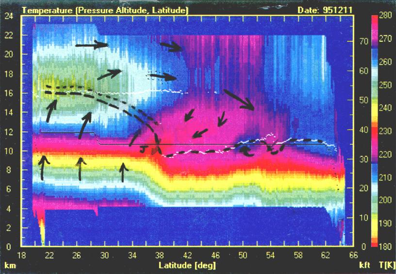
Figure 5. Color-coded air temperature derived from the MTP/DC8
instrument during the 1995 December 11 DC-8 flight from Alaska to Hawaii.
The arrows are subjective interpretations of a
residual circulation that would produce the temperature pattern measured
by the MTP. The "J" at 34.5 degrees latitude represents the sub-tropical
jet. White dots show MTP-measured tropopause
altitudes. The heavy dashed line is the "tracer tropopause" and
is based on ozone and other tracers, described in the text.

Figure 6. Altitude of one isentrope measured by the MTP/ER2 on
a cross-country flight of 1991 November 2, from California to Maine.
The thin red trace is measured (unfiltered) and the thick
black trace is a filtered version meant to simulate synoptic resolution.

Figure 7. Temperature difference, mesoscale measured minus a synoptic scale filtered version of the same data, versus parcel time for the 1991 November 2 ER-2 flight.

Figure 8. Histogram of temperature differences in Fig. 7.

Figure 9. The blue trace is the altitude of the 490 K isentrope surface for the assimilated temperature field (from an archived assimilation data file) for the ER-2 flight of 1991 November 2; the other traces are the same as in Fig. 6. Both plots are with respect to a 19.4 km altitude.

Figure 10. Measured parcel temperature versus assimilated field parcel temperature for the 490 K isentrope surface, for the ER-2 flight of 1991 November 2. This is essentially an estimate of the error of a 2-day back trajectory parcel temperature versus time. Longer back trajectories would likely exhibit greater maximum errors.
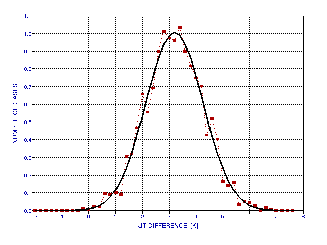
Figure 11. Histogram of temperature differences in Fig. 10.
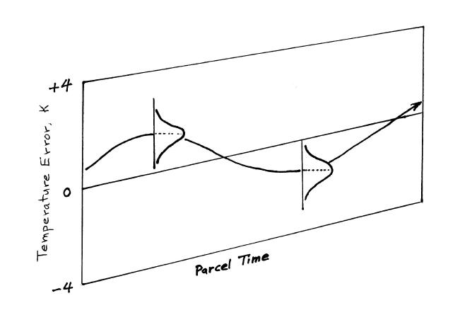
Figure 12. Sketch showing an example plot of "back trajectory temperature error" in relation to histograms for the faster "mesoscale temperature fluctuations."

Figure 13. Power spectrum of temperature fluctuations for ER-2
flight of 1991 November 2, based on MTP isentrope altitudes (red trace).
Model components for synoptic scale (blue) and
mesoscale (green) are added to produce a model fit (thick black) trace.
Spatial wavelengths are given in boxes at the top assuming a fixed wind
speed 24 m/s.
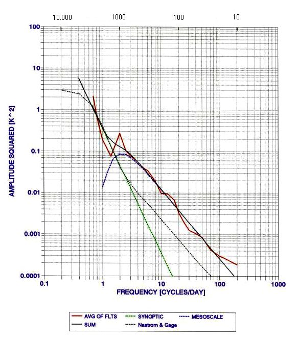
Figure 14. Four-flight average spectrum of MTP/ER2-determined
parcel temperature fluctuations (red) in relation to fits of synoptic scale
and mesoscale components. The dotted line is from Nastrom and Gage's
1985 study of commercial altitude temperature fluctuations. Spatial wavelengths
(in km) are shown at the top.