It is important to be able to fly "isentropically" for the study of chemical processing within mountain wave polar stratospheric clouds, PSCs.  It should be possible to improve the quality of isentropic flight by using a Microwave Temperature Profiler, MTP, remote sensing instrument.  The key to improved isentropic flight is the MTP's ability to measure the altitude of desired isentropes ahead of the aircraft.  Look distances as much as 7 km are possible, allowing for the anticipation of altitude changes up to 90 seconds ahead of time.

Introduction

Air can "experience" polar stratospheric clouds, PSCs, in one of two ways: 1) the air can cool slowly, become supersaturated, and form a large synoptic scale PSC, or 2) the air can flow through a (stationary) mountain wave, and as it is uplifted the air will adiabatically cool and form PSC particles.  Whereas the time spent by an individual air parcel within the mountain wave PSC may be short, if the mountain wave pattern persists for long periods (such as for several days) it can "process" large volumes of air.  Because of the potentially widespread effects that small mountain wave regions may have on the chemical state of the polar vortex, it is important to measure this aspect of their "processing power."

To measure a mountain wave's processing power it is necessary to sample air before it enters a mountain wave PSC, and after it leaves.  It is also important to measure certain properties of the aerosols in the PSC, at the exact locations traversed by the air in the "before" and "after" sampling regions.

How does one trace out the path of air parcels that go through a PSC?  Uplifted air cools, yet maintains its "potential temperature," theta = (1000 mb/BP)0.286.  It is possible to think of  theta-surfaces as delineating air flow streamlines when the  theta-surfaces are viewed in a cross-section that is parallel to the wind direction (and when distances are less than a few thousand kilometers).  Thus, for the purpose of measuring what a particular PSC is doing to an air parcel, it is important to sample air along flight paths that are "isentropic" (at a fixed potential temperature) and parallel to the wind.

Mountain wave PSC's are located at wave crests, or the top of the wavy pattern of isentrope altitude displacement. Unfortunately, mountain waves cause aircraft to undergo erratic altitude changes.  For the ER-2, a field of "wrinkled" isentropes will cause the aircraft to fly up and down with pressure altitude excursions that are approximately 1/2 the amplitude of the isentrope altitude fluctuations.  Thus, isentropic flight through mountain waves is made difficult by the very pattern of vertical displacements that create the PSC.

If isentropic flight is to be part of an experiment's design, some means must be developed for assuring that isentropes can be followed during flight.  The Microwave Temperature Profiler, MTP, is an ideal instrument for providing this assistance.  One channel of a proposed MTP will look 7 km ahead of the aircraft, and locate isentrope surfaces 90 seconds before they are encountered.

This report describes how MTP information could be used to provide "anticipatory flight guidance" to improve the quality of isentropic flight.  The examples used to illustrate isentropic flight strategies assume the use of an MTP that has been proposed for Perseus, which has performance specifications almost identical to an instrument that was flown on NASA's DC-8 in 1992.  The new instrument would be designed for operation aboard the Perseus class of Unmanned Aerial Vehicles, UAVs, under development at the Aurora Flight Sciences Corporation.

Example of a Mountain Wave PSC Encounter

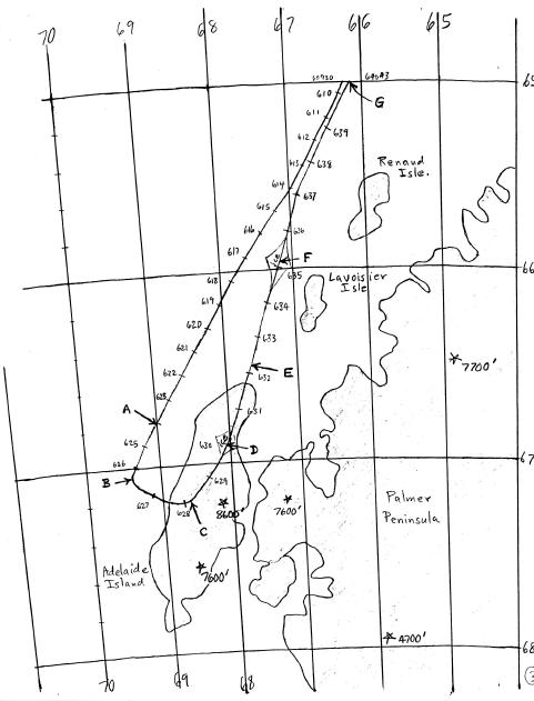
Figure 1 is an "isentrope altitude (flight curtain) cross-section," IAC, for a mountain wave encountered during the 1987 Airborne Antarctic Ozone Experiment.  The isentrope surfaces exhibit distortions with a 1 km peak-to-peak amplitude.  The two main wave crests are 9 minutes of ER-2 flying time apart (115 km).  Large ice crystals (in the 5 to 8 micron diameter data bin) were encountered at locations D and F, which are close to the positions of each wave crest.  Analysis shows that at these two locations the uplifted air had been adiabatically cooled to supersaturation with respect to ice.

Figure 1.  Ground track of ER-2 during flight over a portion of the Antarctic Peninsula where a mountain wave was encountered.

The trace with labels A, B, ... G show the altitude of the ER-2 as it flew through this   field.  Note that the two PSC encounters occur while flying in air having  theta = 415 K, whereas at locations A, B and E, outside the PSC, theta = 425 K. Only non-PSC location G is at theta = 415 K.  To determine if data at location G can be used as either a "before" or "after" reference, for either PSC, a detailed ground track map was prepared, and is presented as Figure 2.

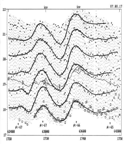
Figure 2.  Isentrope altitude cross-section for the portion of flight indicated by "A" through "G" in the previous figure.

Contours of equal altitude for the 420 K isentrope are shown in Fig. 3.

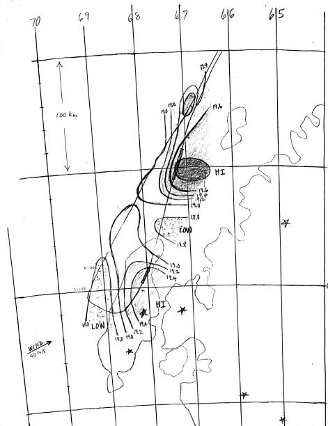
Figure 3.  Altitude isopleths for the 420 K isentrope surface.

These figures show that we have neither "before" nor "after" data for either PSC encounter.  This example illustrates that it can be frustrating to use existing ER-2 data for the study of quantitative effects of specific PSCs on air chemistry.

The three ozone depletion missions in which the ER-2 has participated have employed flight paths that maximize their penetration into the polar vortex.  The direction of flight, therefore, was toward the pole, and back, and in almost all cases this meant that flight was perpendicular to wind direction.  Although experimenters have expressed their desire for flight through a mountain wave PSC parallel to the wind, no such flight has occurred.

MTP Principle of Operation

The MTP is a microwave radiometer (i.e., passive, not radar) which measures the intensity of thermal emission from oxygen molecules along the viewing direction.  The operating frequencies of the proposed MTP/UAV instrument are 55.1, 57.3 and 58.8 GHz (channels 1, 2 and 3).  At these frequencies, and at the pressures and temperatures found at a nominal operating altitude of 20 km, oxygen molecules have an absorption coefficient of approximately 0.14, 0.4 and 0.7 [Nepers/km].  This corresponds to "applicable distances" of 7, 2.4 and 1.4 km.  "Applicable distance" is the distance at which the weighting function for an exponentially-weighted observable is at the 1/e value.  When the source function (air temperature) varies linearly with distance, the observed quantity is exactly equal to the source function at the "applicable distance."

As a first approximation, the MTP-measured brightness temperature can be thought of as the atmospheric physical temperature at locations 7, 2.4 and 1.4 km away from the aircraft along the viewing direction.  For example, if the viewing direction is straight up, then MTP measured brightness temperatures provide an estimate of air temperature at 7, 2.4 and 1.4 km above flight level.  During MTP operation the viewing direction is scanned through a sequence of 10 elevation angles, from -80 to +80 degrees, so the range of altitudes "sampled" is -6.9 to +6.9 km.  This elevation scan, plus a brief calibration, will occur every 14 seconds for the proposed MTP/UAV (the same as for the MTP/DC8), though it could be performed as frequently as every 10 seconds, with a negligible signal-to-noise penalty.  The part of the profile near flight level applies to air that is in front of the aircraft about 7, 2.4 and 1.4 km, while the part of the profile at the upper and lower ends of the altitude coverage applies to air that is ahead of the aircraft by lesser amounts.  (This simple explanation overlooks many second order effects, and it should be noted that a more sophisticated retrieval algorithm is employed for converting observed quantities to desired physical properties.)

By measuring profiles of air temperature versus altitude every 14 seconds, the MTP is, in effect, also measuring profiles of potential temperature,  .  Thus, it is possible to use MTP profiles to locate the altitude of specific isentrope surfaces.  A sequence of MTP measurements of isentrope altitudes is used to construct IAC's.  The IAC in Fig. 1 was constructed from MTP/ER2 data.

How MTP Can Be Used to Select a Best Altitude

An IAC, such as in Fig. 1, can be analyzed to determine where PSCs should exist.  This is possible because the IAC contains information about air temperature at all altitudes in the IAC, and it is possible to calculate the temperature at which the air is saturated with respect to HNO3 and H2O by knowing (or assuming) concentrations for the two molecular species (account is also made for air pressure at the pressure altitude in question).  In other words, by adopting mixing ratios for HNO3 and H2O it is possible to create "saturation cross-section" counterparts to the IAC's, from which it can be inferred that PSCs may exist (super-saturation arguments can also be invoked to refine the PSC predictions).

The IAC in Fig. 1 has been digitized and redrawn as Fig. 4, and subjected to a saturation analysis under the assumption of complete denitrification (HNO3 concentration = 0) and water vapor mixing ratio = 4 ppmv (at all altitudes).

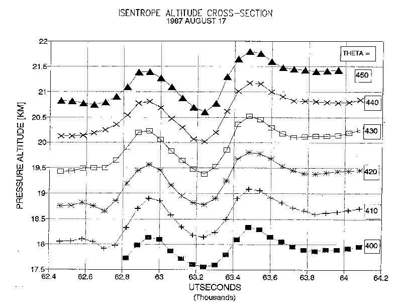
Figure 4.  Digitized version of the isentrope altitude cross-section shown in Fig. 2.

Figure 5 shows where air temperature is colder than the water vapor frost point (the dotted areas), and it is therefore a prediction of where Type III PSCs (mountain wave ice crystal aerosols) could exist.

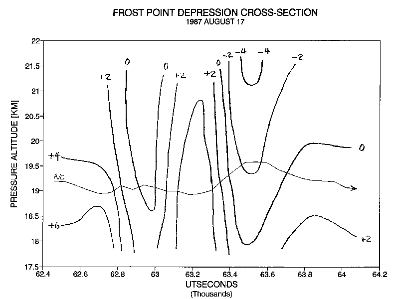
Figure 5.  Isopleths of frost point for the same altitude/time graph as in the previous figure.

The aircraft flight level path is shown crossing into PSCs twice.  By overlapping Fig. 4 into Fig. 5, it will be seen that the two PSC encounters are predicted to occur at the wave crests.

Figure 6 is a record of the FSSP instrument's measurement of particles.

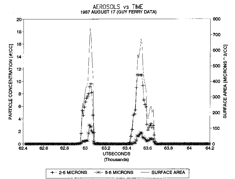
Figure 6.  Particle concentration encoutnered during flight through the mountain wave.

The location of the two particle events corresponds very closely with the MTP-predicted PSC encounters.  Some particles were as large as 5 to 8 microns (diameter).  These can only be ice crystals, sicne there is sufficient HNO3 in the air to produce particles this large.  It is noteworthy that such large particels can grow during periods as short as 10 or 15 minutes, versus the hours and days that conventional microphysical models predict.  (Figure 3 can be used to estimate how abruptly air parcels can be forced upward and adiabatically cooled and still produce large particles.)

Figure 5, a "frost point depression flight curtain cross-section," can be thought of as a "predicted PSC cross-section."  Such cross-sections could be produced in real time from an MTP/UAV transmitting data to a ground station.  It could be used to help decide which altitudes may have the greatest scientific payoffs for sampling during subsequent up-wind and down-wind passes.  For the case depicted in Fig. 5, "the higher the better," at least up to 21.5 km.  On other occassions the PSC might be found in a layer, and the predicted PSC cross-section could be used to guide flight to altitudes having the densest PSC.

How MTP Can Improve Isentropic Flight

Isentropic flight requires knowledge of the isentrope altitude cross-section, IAC, ahead of the aircraft as well as in the vicinity of the aircraft.  If the pilot's task is to fly along the theta = 500 K surface, for example, the task for MTP would be to advise the pilot about the altitude of the 500 K isentrope 1.4, 2.4 and 7 km ahead of the aircraft.  The IAC produced when the aircraft was 1.4 km behind it's present location can be used to specify where the 500 K surface is in the aircraft's vicinity (the same can be done for other surfaces).  If the desired isentrope ahead of the aircraft is higher than the aircraft, then the aircraft should be climbing.

Another way of viewing this task is to state that the MTP is trying to monitor the slope of the isentropes in the region between the aircraft's current position and locations slightly ahead of the aircraft, along the flight path.  This can be treated as equivalent to measuring the horizontal and vertical gradients of air temperature.  The vertical gradient is called lapse rate,  T/ z.  MTP can measure  T/ z at 1.4, 2.4 and 7 km ahead of the aircraft.

There are several ways of measuring the horizontal gradient.  The recent trend of in situ air temperature, converted  to a standard, or nearby, altitude (using MTP's  T/ z) can be used to assess the horizontal gradient for a region immediately behind the aircraft.  This method would have good precision, but it would apply to air on the wrong side of the aircraft's flight path.  A better method of measuring the horizontal gradient is to compare MTP's measured air temperature while viewing the horizon 1.5 and 3 km ahead of the aircraft.  Though less precise, this method would at least assess the horizontal gradient ahead of the aircraft.

Combining the horizontal and vertical temperature gradients yields the slope of nearby isentropes ahead of the aircraft.

Implementation Example

How might MTP isentrope information be conveyed to the UAV pilot?  I will assume that MTP data is telemetered to a ground station, where real-time analysis is performed by an MTP analysis computer.  This MTP analysis computer could be monitored by an MTP experimenter, or it could be programmed to issue audible alerts to the UAV pilot automatically.  The audible alert mode could be initiated at the start of each isentropic flight segment, when an operator would enter the desired isentrope value to the MTP computer.  As a minimum, the computer would display the current  , and the current isentrope slope, in degrees.  The computer could display the altitude difference between the UAV and the altitude of the desired isentrope at 1.4, 2.4 and 7 km ahead of the aircraft.

It is worth noting the similarity of flying a glideslope during landing and "flying" a sloped isentrope.  An audible beep might be used to encode altitude error information.  For example, the interval between beeps of one type could signify how far above the desired isentrope the aircraft was flying, while the interval between beeps of another type could signify the magnitude of the altitude error below the desired isentrope.  When the altitude error is within a pre-set tolerance, no beeps would occur.  When isentrope curvatures are present, such as in Fig. 11 (which is rare), a verbal message could be issued (perhaps automatically by the MTP computer), such as:

 Isentrope curvature:  prepare for abrupt decrease of isentrope from its extrapolated location.

Since it is possible that there would be a problem of false alarms with an automated MTP analysis computer, keeping humans in the loop is clearly prudent at the outset.

Characteristics of Typical Mountain Waves

Estimates of isentrope slopes can be made from Fig. 1 (or Fig. 4), which is an example of a "gentle," non-turbulent mountain wave.  The   = 420 K isentrope has a maximum slope of 1.5 degrees.  A Perseus A or B type UAV flies at approximately 75 [m/s].  (With this speed, which is approximately 36% that of the ER-2, the time scale of Fig. 1 should be stretched by a factor 2.8, so that a 9 minute spacing between wave crests would be 25 minutes for a UAV).  At this speed a 1.5 degree slope corresponds to a climb rate of 2.0 [m/s].

Air moving horizontally along such a sloped surface at 40 [m/s], which is the horizontal wind speed for this particular example, would have a vertical velocity of 1.1 [m/s].  Thus, for this example, a UAV would need a climb rate that could be as high as 2.0 + 1.1 = 3.1 [m/s].

These numbers assume that the IAC is oriented parallel to the wind, which it isn't.  But, according to Fig. 3, this particular mountain wave event has approximately circularly-symmetric shapes (the way I've drawn them, admittedly), so an IAC parallel to the wind would yield similar isentrope slopes, and similar required climb rates.

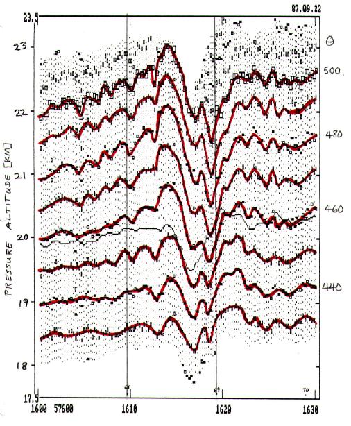
Figure 7.  IAC for the largest mountain wave encountered by the MTP, during the 1987.09.22 flight over the Antarctic Peninsula.

Figure 7 is the first IAC produced with the MTP instrument, and by chance it yielded one of the most dramatic mountain waves in the MTP archive.  This IAC is over Antarctica on 1987 September 22.  Later analyses showed that a wave feature similar to this one, though slightly less dramatic, was present at the same location during the previous two ER-2 flights (on September 20 and 21).  Thus, this mountain wave feature lasted for 3 days, at least, and possibly many more.  Large volumes of air must have passed through the wave feature.

The peak-to-peak vertical displacements increase in going from low   values (700 meters for   = 430 K) to high   values (1800 meters for   = 480 K).  Considering the   = 450 K isentrope, which is close to the ER-2's flight level, the maximum slope is 2.7 degrees.  For a UAV air speed of 75 [m/s], a UAV would need to climb 3.5 [m/s] in the absence of winds.  The MMS horizontal winds were measured to be 35 [m/s], so there must have been a vertical wind component of approximately 1.6 [m/s].  The UAV's rate of climb requirement would have been 2.0 or 5.1 [m/s], depending on wind direction, for the steepest slope region.

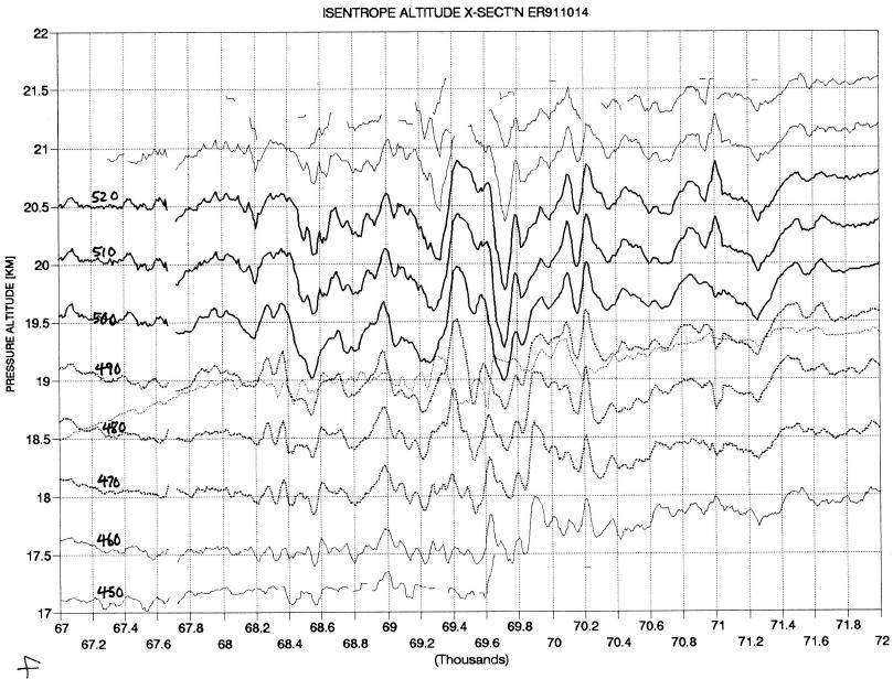
Figure 8.  IAC for an ER-2 flight on 1991.10.14 over Alaska.

Figure 8 is an IAC for another mountain wave, encountered in 1991 during the Arctic Airborne Stratospheric Expedition II.  The greatest isentrope displacements, at approximately 69.4 ksec, occur during flight over 16,000 foot Mt. Blackburn, in south-eastern Alaska.  The dotted line is the ER-2 altitude.

I have performed an analysis of "flight path Richardson Number" for this flight period, and the entire region depicted in Fig. 8 is dynamically unstable.  Ri has values that are typically in the range 0.5 to 2 throughout most of this region (compared with values of about 2 to 5 during a later portion of the flight that was "smooth").  The low Ri values are apparently due to high values of vertical wind shear created within an inversion layer, which happened to be close to the ER-2's flight altitude most of the time.  Moderate clear air turbulence, CAT, is encountered between 69.4 and 69.6 ksec.  About 5 minutes before the CAT started (from 69.0 to 69.2 ksec), Ri   1/4, the magic threshold for producing CAT.

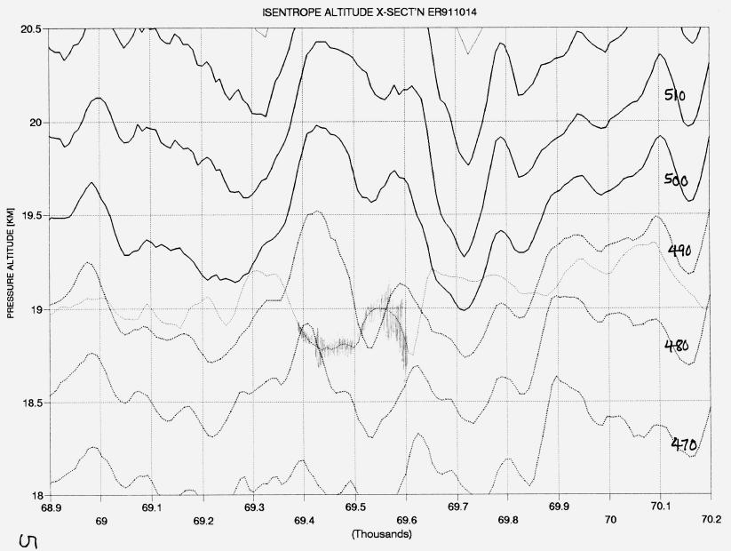
Figure 9.  Zoom of most "active" portion of the previous IAC.

Figure 9 is a "zoomed" version of the portion exhibiting the largest isentrope displacements, in the vicinity of the CAT.  I note here that the CAT region is anomalous in having lapse rates close to adiabatic, which is quite rare for in the archive of MTP data.  The regions surrounding the CAT patch have high positive lapse rates (+5 [K/km]), which is also quite rare.  This is obviously a dynamically unstable mountain wave, and can serve as a worst case example for simulating the feasibility of isentropic flying.

Steep slopes occur in many parts of the IAC in Fig. 9.  For example, the theta = 480 K isentrope, at 69.86 ksec, exhibits a slope of 3.0 degrees (and this is outside the turbulent region).  The horizontal wind in this region is 23 [m/s].  If the wind were in the plane of the IAC cross-section, the 3 degree slope would imply vertical wind velocities of 1.1 [m/s].  The Meteorology Measurement System, MMS, measured vertical winds in this region of 1.5 [m/s], which implies that isentrope slopes for a cross-section that was closer to parallel to the wind would exhibit isentrope slopes of about 4 degrees.

A method has been devised for obtaining an IAC that has a greatly improved temporal (horizontal) resolution, but it is only valid over a shallow range of altitudes, and beyond this shallow layer the altitude accuracy is degraded considerably compared to the accuracy that MTP provides.  The method is based on MMS 1 Hz air temperature and pressure altitude readings.  The key assumption that must be made is that the MTP-measured lapse rate, dT/dz (which is readily convertible to the parameter that is actually used, dtheta/dz), changes slower than the MTP cycle time of 9 seconds.  This assumption should be safe, since dT/dz changes slowly from MTP cycle to cycle.  With this assumption, it is possible to calculate the altitude of nearby isentropes from each 1-second MMS reading of theta and pressure altitude.

If the lapse rate is derived from the MTP 58.8 GHz channel's +10 and -11 degree measurements, then the lapse rate applies to a layer approximately 500 meters thick (FWHM), centered on the aircraft altitude.  Thus, any isentrope altitudes derived from the combination of MMS and MTP data should be valid throughout the 500 meter thick layer, and possibly for a much larger layer.  It is possible to use MTP data to calculate dtheta/dz for a range of layer thicknesses, and then, through an iterative process, use the appropriate dtheta/dz to calculate each isentrope's altitudes more accurately.  (For the present analysis, I have not done this.  Instead, a simpler empirical formula, which is not worth describing here, has been derived for improving the validity of the lapse rate assumption for more distant isentropes.)

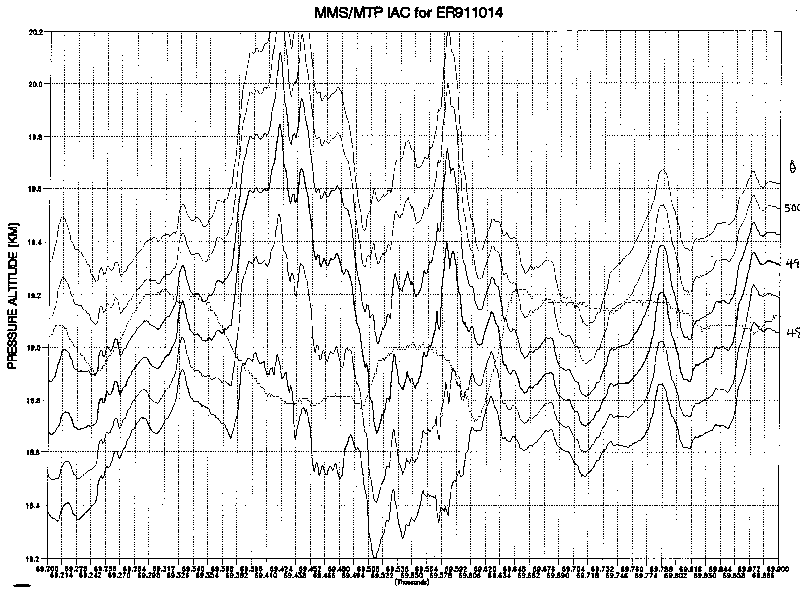
Figure 10.  IAC detail of region in previous figure, showing isentrope surfaces 5 K apart.

Figure 10 is a MMS/MTP IAC for a zoomed portion of the previous figure.  It has been smoothed to have an approximate temporal resolution of 3 seconds (600 meters horizontally).  The vertical lines are 14 seconds apart, which corresponds to the present MTP's farthest "look distance" of 3 km.  (The new MTP/UAV will see twice as far, or the distance of two vertical lines in Fig. 11.)  This greater temporal resolution is probably only important for especially active mountain waves, such as the present one.  The moderate CAT encounter begins at 69.38 ksec, where the isentropes slope upward steeply.  The CAT ends abruptly at 69.61 ksec, where the isentropes slope down steeply.  Probably these two isentrope features, and everything in between (which is turbulent), can be ignored for the present analysis, since mountain wave CAT of this magnitude is rare.

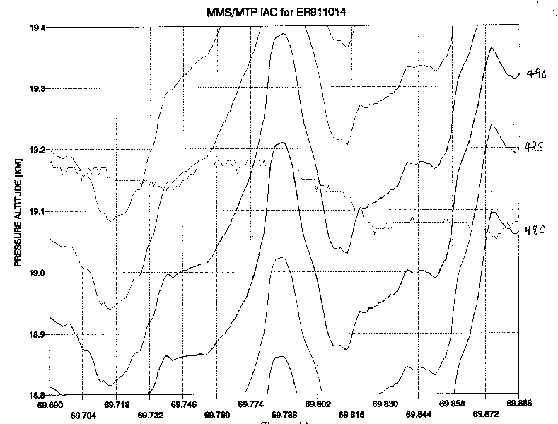
Figure 11.  IAC with even greater detail of region in previous figure.

Figure 11 is a zoomed version of an "upward thrusting" feature in the previous figure that is encountered after the CAT patch.  It is not turbulent, but may still be unusual due to the dynamic instability of the region, generally.  It can thus serve as a possible "worst case" situation for isentropic flying.  The isentropes near flight level on either side of 69.788 have slopes of about 10 degrees.  According to MMS, the vertical wind was +3 and -3 [m/s] at these locations.  Thus, for an IAC that is parallel to the wind direction the isentrope slopes would apparently be about 7.5 degrees (23 [m/s] times tangent 7.5 degrees = 3 [m/s]).  The slopes on either side of the peak are about the same.

If the wind were from left-to-right in Fig. 11, and the if the UAV were flying at 75 [m/s] in the same direction (i.e., a tail wind), the rate of climb requirement for isentropic flight would go through a maximum value of +7 [m/s] on the climb to -13 [m/s] during the descent.  If the wind were in the other direction, the rates of climb requirements would be +13 [m/s] and -7 [m/s].

A UAV travelling at 75 [m/s] through the  -field in Fig. 11 would have to adjust its rate of climb by 20 [m/s] in going from the region of maximum slope on one side to maximum slope on the other side, in order to fly isentropically.  This abrupt change in rate of climb must be executed in the time it takes to fly about 3 km, which is 40 seconds for a 75 [m/s] UAV.  Surely, it would be helpful to know ahead of time that a change from about +10 [m/s] to about -10 [m/s] is to be made in the span of about half 40 seconds, as Fig. 11 shows would be required.

An MTP aboard the UAV could provide updates of the isentrope location at the 1.4, 2.4 and 7.0 km distances (19, 32 and 93 seconds of UAV flying time).  With this guidance it should be possible to anticipate rate of climb needs instead of reacting after the fact, as would occur without an MTP.

Importance of Flying With a Tail Wind

Each aircraft will have its own "rate of climb versus flight level" limitation.  The Perseus A aircraft's maximum rate of climb is currently estimated to be about 4 [m/s] while flying at 20 km.  Whereas the previous discussion applies to UAVs, generally, the remainder of this section is focused mainly on the potential problems of using the Perseus A for flying isentropically.

For the IAC in Fig. 1, having slopes of 1.5 degrees, in the absence of winds the UAV would need rates of climb of 2.0 [m/s], which is well within the capability of Perseus A.  Considering the 40 [m/s] wind that actually existed, for a tail wind pass the 1.1 [m/s] vertical wind component would relax the UAV's rate of climb requirement to 0.9 [m/s].  But for a head wind pass, the rate of climb requirement is 3.1 [m/s], which is also within the Perseus A's nominal capability.

The mountain wave in Fig. 7 has rate of climb requirements of 2.0 [m/s] with a tail wind, and 5.1 [m/s] with a head wind.  Whereas this wave could not be flown properly during head wind passes, it can be flown well during tail wind passes, according to the same arguments used for the previous mountain wave case.

Let's try to estimate altitude errors during a headwind flight leg.  The longest 2.7 degree slope is 12.8 km long, which Perseus A would fly in 171 seconds.  If the rate of climb was 4 [m/s] instead of the desired 5.1 [m/s] for this 171 seconds, an error of 190 meters would be accumulated.  The error in   would grow to 3 K during this time.  If an MTP/UAV were used to give Perseus a head start on the climb, these errors could be reduced to almost 1/2 their former values, i.e., 100 meters and 1.5 K of  .  These errors strike me as being acceptable in the context of the scientific objectives.  We conclude from this mountain wave example that the downwind flight segments could be flown isentropically and the headwind segments would accumulate acceptable errors.

The isentrope feature in Fig. 11 could not be flown isentropically in either direction by Perseus A, since the required rates of climb of 7 and 13 [m/s] are far in excess of the 4 [m/s] Perseus A capability.

It may be possible for Perseus A to climb at faster rates for brief periods, which might merit consideration. It may also be possible to modify the Perseus A design to permit short bursts of power for accommodating the occasional steep isentrope.

A more reasonable approach is to minimize altitude errors using MTP to get a "head start" on the isentrope climb.  As mentioned for the previous mountain wave case, MTP information about isentrope altitudes 7.0 km ahead of the aircraft would enable altitude errors to be reduced to half their value for highly sloped features with horizontal extents as great as about 7 km.  For example, at time 69.760 ksec MTP would be able to notify the Perseus A flight controller that the present isentrope is 300 meters higher at 6 km ahead of the aircraft, requiring a 4 [m/s] climb to reach it.  If action is taken quickly, the isentrope could be followed thoughout its wild variations with altitude errors of approximately 50 meters.

A better quantitative assessment of how well isentropes could be flown with an MTP instrument requires more detailed simulations, that incorporate detailed UAV flight response characteristics and pilot control capabilities.  Such a study is beyond the scope of the present analysis.

One of the purposes of this report has been to determine whether or not a more detailed analysis is required.  Based on the results reported here, showing that an MTP instrument could enable Perseus A to fly isentropically though all mountain waves considered, I conclude that a more detailed study is warranted.

Summary

Typical mountain wave isentropes are sloped 1 or 2 degrees, and depart 300 to 500 meters above and below their undisturbed altitude.  When a region is "dynamically unstable" (due to high values of vertical wind shear) slopes as high as 8 degrees may be encountered over short distances.  Unstable conditions can also produce abrupt changes of isentrope slope (i.e., isentrope curvature) on timescales of 40 seconds.

Use of a microwave temperature profiler instrument aboard a UAV can provide real-time measurements of the slope of isentrope surfaces ahead of the aircraft, as well as warnings of abrupt inflections of the isentrope surface.  A proposed MTP/UAV instrument could provide information about isentrope altitudes and inflections 1.4, 2.4 and 7 km ahead of the aircraft along the flight path.  This translates to 19, 32 and 93 seconds of advance warning, assuming typical UAV flight speeds of 75 [m/s]. It is theoretically possible to use this advance information to fly along isentrope surfaces with a tolerance of approximately 100 meters for most mountain wave cases.

The very active mountain waves can pose a problem for isentropic flight.  However, the horizontal extent of highly distorted isentropes is so short that an MTP/UAV instrument can characterize them well enough to assure 100 meter tolerances during isentropic flight.

Detailed simulations should be performed using a more thorough performance characterization of the Perseus A, and using a greater number of mountain wave cases.  Isentrope following errors should be evaluated for their scientific impact.  Modifications to either the UAV or MTP should be considered, to see if there are ways to improve isentrope following performance for the more difficult mountain waves.

If future studies confirm that it is possible for almost all mountain waves to be flown through isentropically, this would mean that we are poised for achieving an important breakthrough in airborne studies of stratospheric chemistry.

This site opened:  March 2, 2000.  Last Update: February 27, 2002