It is now possible to measure the temperature field of the planetary boundary layer with mesoscale spatial sampling using a microwave radiometer aboard an airplane.  This report illustrates what is possible using actual measurements from the Microwave Temperature Profiler, MTP, which is installed on a semi-permanent basis in the NASA DC-8 aircraft.

Introduction

The question sometimes arises "Can the airborne Microwave Temperature Profiler work at planetary boundary layer altitudes?"  The answer is "yes" which surprises some  because all published MTP results are for flight at altitudes in the 10 to 21 km region.  Surely, some compromises on low-altitude performance had to have been made in designing the MTP for high altitudes, it is assumed.  However, the compromises are minimal, and the high-altitude MTPs, especially the MTP/DC8 (aboard the NASA DC-8), work just fine at low altitudes.  Low altitude performance is changed in the sense that the altitude region for which useful T(z) can be retrieved is smaller, being inversely proportional to ambient pressure.  However, the altitude resolution is better.  This web page presentes results of a PBL flight.

Location

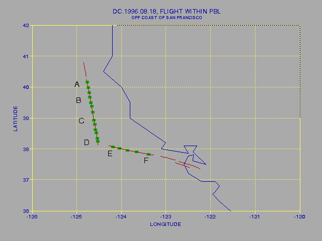
On August 18, 1996, the DC-8 flew over the ocean at low altitude just west of San Francisco.

Figure 1.  Ground track for two flight segments at constant altitudes of 0.3 km, A to D, and 0.9 km, E to F.

The figure shows two level flight tracks at 0.3 and 0.9 km altitude, just prior to landing at the Ames Flight Research Center's Moffett Field.

Temperature Profiles

Figure 2.  T(z) profiles from 90-second averages of MTP retrieved temperatures, corresponding to flight between points A and B in Fig.1.  The thick horizontal line indicates the DC-8 altitude.  The Y-axis is pressure altitude.

Profile #1 in Fig. 2 is the northernmost of the set of 5 profiles, and since it is noticeably colder than Profile #2 we may assume that during the descent that occurred just before Profile #1 was taken the warmest part of the inversion layer, at 1.0 km, was even cooler than shown in Profile #1.  This will be confirmed in a later figure, in the validation section.  The trend for a warming inversion layer continues during the 8 minutes represented by this figure.

Figure 3.  T(z) profiles corresponding to flight between points B and C in Fig.1.

This figure shows a stabilizing in inversion layer temperature during this 8-minutes of flight data, located in the middle of the first, southbound flight track.

Figure 4.  T(z) profiles corresponding to flight between points C and D in Fig.1.

During the first 4 profiles, labelled 11 through 14, the inversion layer cools about 2 K, followed by a 1 K warming.
 

Figure 5.  T(z) profiles corresponding to flight between points E and F in Fig.1, which is the second level flight leg with the DC-8 at a new altitude of 0.9 km, near the inversion layer top .
The ascent to 0.9 km should have brought the DC-8 to within 0.1 km of the inversion layer top, the warmest altitude of the PBL, and the 5 T(z) profiles in this figure confirm this prediction.  A warming trend within the inversion layer continues during this southesaterly flight segment.

Validation

Since it is not possible to use radiosondes to validate the MTP profiles (since there are none at the ocean locations of this flgiht), we must rely upon the in situ air temperature measurements during ascent and descent portions of the flight.  Since MTP has evidence for the presence of mesoscale dynamics over 50 km distances, care must be taken in making the OAT verus MTP comparisons.  The next figure shows the relevant ascent and descent portions of in situ air temperature, or Outside Air Temperature, plotted versus altitude, OAT(z).  It also includes 3 MTP profiles taken close to the ascent and descent regions.

Figure 6.  The thick black traces are OAT(z) profiles, and the thin colored traces are MTP retrieved T(z) profiles.  The cold arm of the OAT(z) trace corresponding to the descent just prior to the first MTP profile in Fig. 2 ((i.e., it is located just north of Point A in Fig. 1).  The warm arm of the OAT(z) trace is for the beginning and ending portions of the flight, located southeast of Point F in Fig. 1.  The 3 MTP profiles are from the previous figures, and retain their numerical identification.

In this figure we are able to compare MTP retrieved T(z) with OAT(z) for two regions, near Point A and near Point F (in Fig. 1).  Remember that the trend for MTP profiles 1 through 5 in Fig. 2 is for increasing warmth at inversion layer altitudes while flying south.  Extrapolating backwards would produce a predicted T(z) in approximate agreement with the cold arm of the OAT(z) trace.  The warm arm of the OAT trace was taken at three locations.  Below 1 km the warm arm of OAT(z) is between Point D and E; the portion between 1 km and 1.7 km is near Point F, and the warm arm of OAT(z) extending down from the top of the figure is from a region near the airport (taken during the beginning of the flight), located southeast of Point F.  The MTP profile labelled 21 is close to Point F, and it is compatible with the OAT(z) warm arm.

Temperature Field

Figure 7.  The bottom two traces are MTP-based temperature at altitudes 0.5 km and 1.0 km during the two flight segments.  Each symbol is a 90-second average.  The dashed blue trace is dT/dz  at 0.6 km.

This figure illustrates the temperature changes noted in the above commentary.  Note the good "precision" of all measurements.  For 90-second averages, corresponding to approximately 15 km of ground track distance, MTP retrieved temperature exhibits a stochastic scatter of approximately 0.1 K.  Lapse rate is measured at a remote altitude, in this case in the middle of the inversion layer, with a stochastic scatter of approximately 0.3 K/km, or 3% of the adiabatic lapse rate.

Figure 8.  Color-coded temperature on a time/altitude field.  The portion to the kleft of the dark vertical band corresponds to flight from Point A to D, while the portion to the right corresponds to flight between Points E and F.  (Disregard the colors at 0 km.)

This figure perhaps has greater visual appeal, but it contains in one image the same information found in the previous several figures.  The altitude quantization is apparent, as is the temporal averaging interval (90-seconds).   For those with experience in mesoscale PBL meteorology dynamics there may be patterns present that I do not recognize.  My competence ends at this interface between measurment and atmospheric theory, so I cannot state whether measurements like these have scientific value.

This site opened:  January, 8, 2000.  Last Update: January 27, 2000